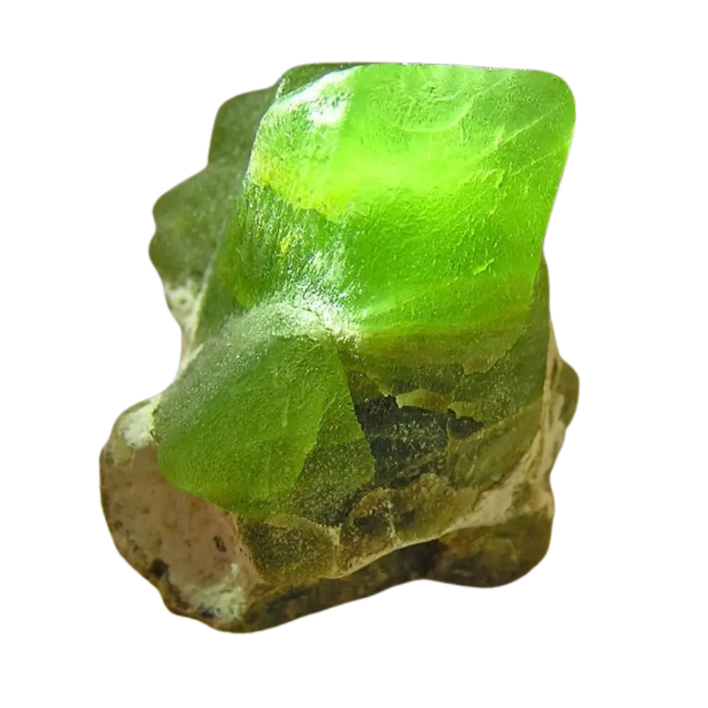
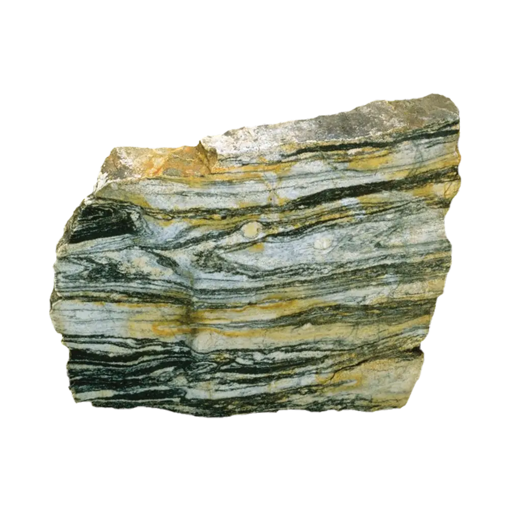
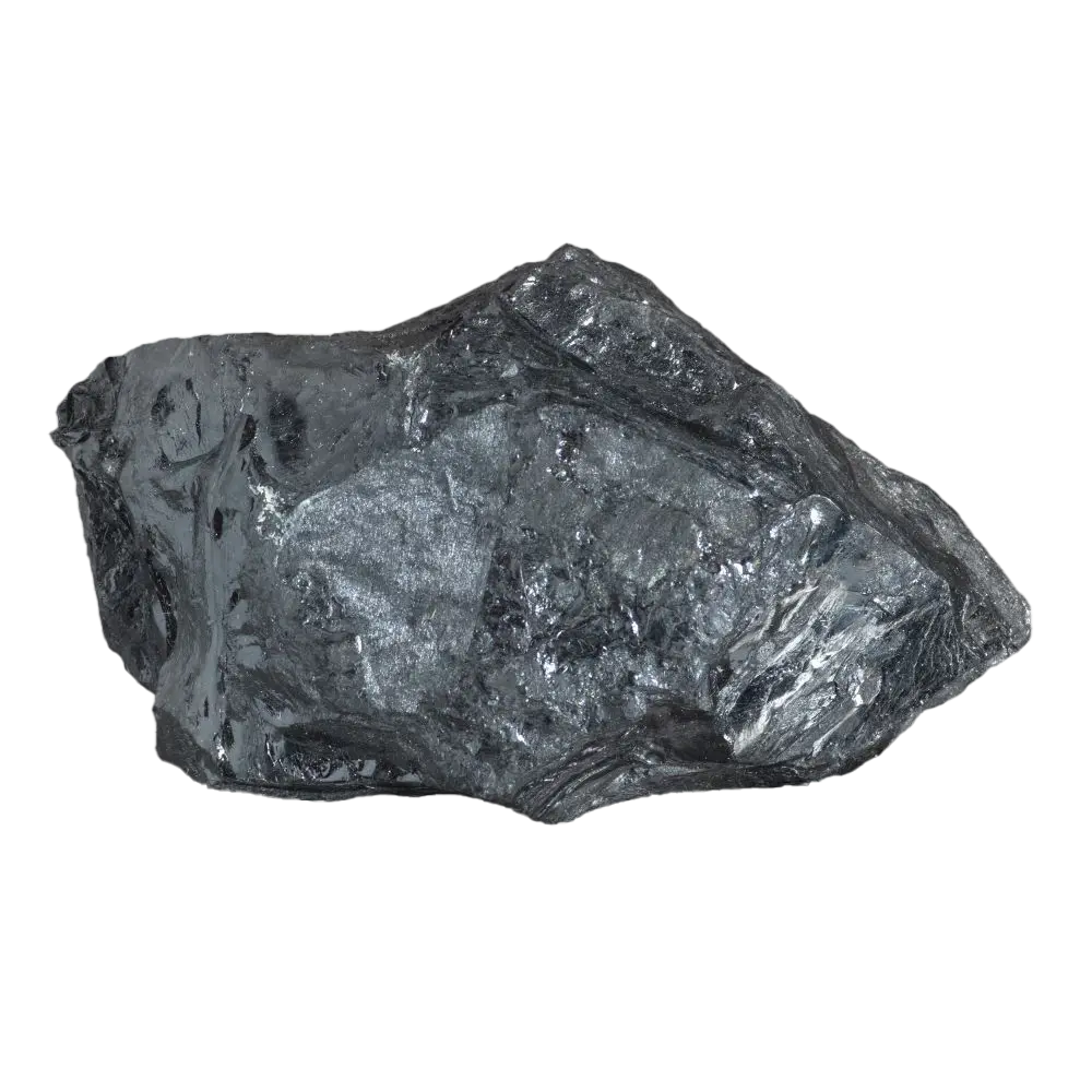
Introduction

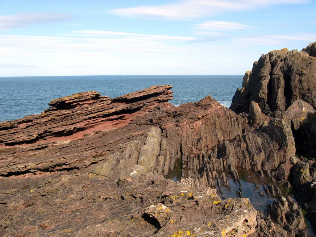
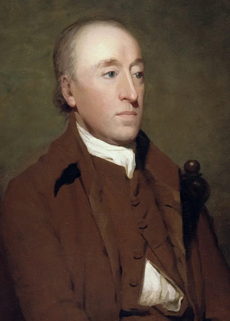
On a fine day in June 1788, three men rowed a small boat along the Berwickshire coast of Scotland and, without quite realising it, gave geology one of its clearest demonstrations of deep time. James Hutton, a farmer and physician turned geologist, wanted to show his friends John Playfair and Sir James Hall a rock junction he was sure existed. At Siccar Point they found it: steeply upended grey rock, sheared off flat, and lying across the top of it a younger set of red beds. Playfair later wrote that “the mind seemed to grow giddy by looking so far into the abyss of time.” Many of the most familiar boundaries on the geologic time scale coincide with major biological, climatic or geochemical changes: a surge of oxygen, a planet frozen to the equator, an explosion of animal life. Many Phanerozoic boundaries are pinned to a specific physical reference section, while others, especially in the Precambrian, are defined chronometrically.

This piece is the deep-time companion to Geoscopy’s foundational pillar, Geology, Explained. Where that page covers how the Earth works, this one covers when, 4.54 billion years of it, and how we know.

What the geologic time scale actually is

Strip away the names and the time scale is a nested hierarchy. From the largest slices of time down to the smallest, the ranks are: eon, era, period, epoch, and age. There are four eons. The current one, the Phanerozoic, splits into three eras, Paleozoic, Mesozoic, Cenozoic. Each era holds several periods (the Cambrian, the Jurassic, and so on). Periods hold epochs, and epochs hold ages. We live in the Phanerozoic Eon, the Cenozoic Era, the Quaternary Period, the Holocene Epoch, and, since 2018, the Meghalayan Age.

Every time unit has a twin. When you talk about the time, “the Cambrian Period lasted about 52 million years”, you are using a geochronologic unit. When you talk about the rocks laid down during that time, “the fossils in this Cambrian System outcrop”, you are using a chronostratigraphic unit. The pairs are eon–eonothem, era–erathem, period–system, epoch–series and age–stage. The rocks are the physical record; the time is what we read off them. Geologists keep both vocabularies because you date the time by studying the rock.

Someone has to maintain all this. That job belongs to the International Commission on Stratigraphy (ICS), the largest body within the International Union of Geological Sciences (IUGS). The ICS publishes the International Chronostratigraphic Chart, the master document every geologist works from. It is revised whenever a boundary is redefined or a date sharpened. The version current as of this writing is 2026/06, released on 20 June 2026, which refined the numeric ages of two Triassic stages (the base of the Anisian to 247.0 Ma and the base of the Olenekian to 250.8 Ma) and one Permian stage (the base of the Wuchiapingian to 259.857 ± 0.084 Ma). The ICS makes the chart freely downloadable and maintains translations of current and recent editions in numerous languages.; it is reproduced below with attribution (© ICS, Cohen et al. 2025, updated). If you remember one source from this article, make it stratigraphy.org.

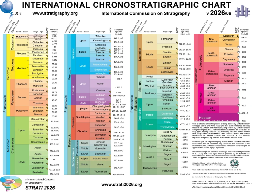
A note on spelling, because both forms are common: the geological time scale and the geologic time scale are the same thing. “Geologic” is the more common American form; “geological” is standard British usage. Nothing scientific hangs on the difference.

How the scale was built before anyone knew a single date

Much of the Phanerozoic framework, the succession of periods and the three major eras, was assembled in the nineteenth century by people who had no way of measuring a single year. They had no radioactivity, no isotopes, no numbers at all. They had rocks, fossils, and two ideas.

The first idea is superposition: in an undisturbed stack of sedimentary layers, the ones on the bottom are older than the ones on top. Obvious once stated, and first set down clearly by Nicolas Steno in the 1600s. The second, and more powerful, is faunal succession: fossil assemblages occur in a repeatable succession through stratigraphic sequences, allowing rocks in different places to be correlated. That was the discovery of an English canal surveyor named William Smith, who noticed while digging canals that each rock layer carried its own signature fossils, and that the layers always came in the same sequence.

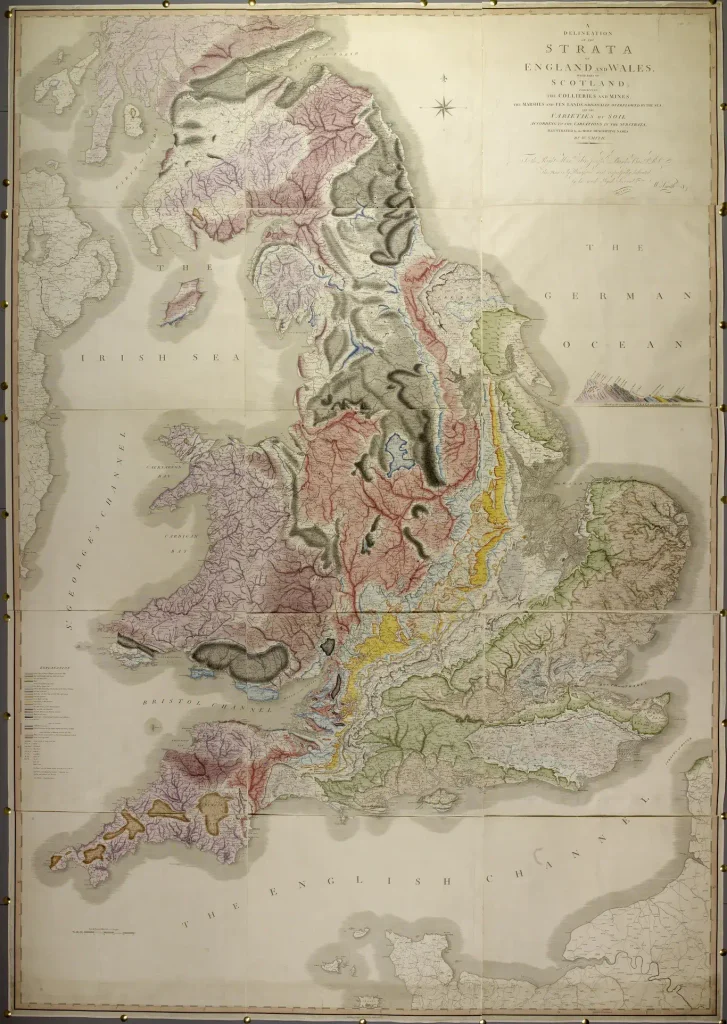
Smith turned that principle into the first geological map of an entire nation, published in 1815. It showed that characteristic fossil assemblages could be used to recognise and correlate particular strata across the landscape. That practical trick, correlation by fossils, is still the backbone of the working time scale two centuries later.

The nineteenth century then filled in the periods, often through fierce academic warfare. In France, Georges Cuvier and Alexandre Brongniart mapped the fossil-bearing strata of the Paris basin and showed that whole faunas could vanish. In Britain, Adam Sedgwick worked upward from the ancient rocks of Wales and named the Cambrian; Roderick Murchison worked downward and named the Silurian; and their claims overlapped so badly that the two men, once close friends, feuded for the rest of their lives over who owned the disputed middle ground. The quarrel was only resolved in 1879, after both were dead, when Charles Lapworth carved the contested interval out and named it the Ordovician, a diplomatic third period slotted neatly between the other two. Charles Lyell, meanwhile, subdivided the youngest rocks into epochs by counting how many of their molluscs were still alive today.

In 1841 William Smith’s nephew John Phillips took the decisive step. Working through the fossil record of Britain, he found two horizons at which the fauna was replaced wholesale, and used them to group the systems into three great eras: the Paleozoic (‘ancient life’, a name Sedgwick had coined in 1838 for a narrower slice, which Phillips widened), the Mesozoic (‘middle life’) and the Cenozoic (‘new life’), both his own coinages. In 1860 he drew the first diversity curve for the fossil record, and the two crashes stand out on it. Phillips had no idea what caused the crashes. We now recognise those boundaries as two of the “Big Five” mass extinctions: the end-Permian and the end-Cretaceous. Phillips had effectively used major turnovers in the fossil record to delimit eras before their causes, or even the modern concept of mass extinction, were understood. The scale’s biggest divisions were forced on geologists by catastrophes written into the rock, decades before anyone knew what a mass extinction was.

How numbers were finally put on it

The Victorians built the sequence but could not date it. The Earth might have been twenty million years old or two billion; the physicists and the geologists argued bitterly, and the physicists, led by Lord Kelvin and working from how fast a molten Earth would cool, kept the numbers small: tens of millions of years at most. What broke the deadlock was radioactivity.

In the early 1900s Ernest Rutherford proposed in 1904–05 that accumulating decay products could serve as a clock, and in 1907 Bertram Boltwood produced the first uranium-lead ages. A young geologist named Arthur Holmes ran with the idea, and in 1913, aged 23, published The Age of the Earth, arguing from uranium-lead ratios that some rocks were well over a billion years old. He spent the next four decades refining the method, becoming one of the leading advocates for turning deep time into a quantitatively dated history.

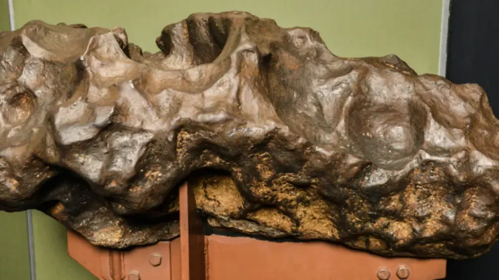
The clinching number came in 1956. At Caltech, Clair Patterson had built an ultra-clean laboratory, because lead contamination was everywhere and lead was exactly what he needed to measure. In his 1956 paper “Age of Meteorites and the Earth,” Patterson analysed lead isotopes from five meteorites, three stony meteorites and troilite from two iron meteorites, including Canyon Diablo. Their Pb-isotope compositions defined an isochron corresponding to 4.55 ± 0.07 billion years. He then showed that terrestrial lead, including lead from modern ocean sediment, was consistent with the same isotopic evolution, linking the meteorite age to Earth.

How radiometric dating actually works

You do not need equations to understand the clock, so here it is in words first. Certain atoms are unstable. A “parent” atom decays into a stable “daughter” atom at a characteristic rate that, for the decay systems used in geochronology, is effectively insensitive to ordinary geological temperatures and pressures, a property we can measure precisely in the lab. The half-life is the time for half the parent atoms in a sample to decay. Uranium-238 has a half-life of about 4.5 billion years; uranium-235, about 704 million. So if you can measure how much parent is left and how much daughter has piled up, and you know the half-life, you can solve for how long the clock has been running.

The workhorse for the deepest time is uranium-lead dating of zircon. Zircon is a tiny, tough crystal that forms in cooling magma. When it crystallises, it readily incorporates uranium but generally excludes lead when it crystallises, so most lead in a pristine zircon is radiogenic after the crystal formed. That makes zircon exceptionally useful as a geological clock, provided later Pb loss, inheritance and common lead are recognised and tested. Zircons also survive being eroded, buried, heated and re-buried, which is why they carry the oldest dates we have. For readers who want the actual relationship, it is D = P(e^λt − 1), where D is measured daughter atoms, P the surviving parent, λ the decay constant, and t the age. That one line underpins the whole numbered scale.

A second method, argon-argon dating, tracks the decay of potassium-40 to argon-40 and is superb for dating volcanic ash layers, which matters enormously, because a datable ash bed sandwiched between fossil-bearing rocks lets you hang a real number on a fossil boundary. Between them, U-Pb and Ar-Ar dating turned the Victorian sequence into a calibrated scale.

How sure are we? Sure to within stated error bars. The end-Permian extinction is dated to 251.9 million years ago; the end-Cretaceous to 66.0 million years; individual high-precision zircon dates now carry uncertainties of a few tens of thousands of years on events a quarter of a billion years old. The oldest dated fragment of Earth is a zircon from the Jack Hills of Western Australia, confirmed by John Valley’s team at the University of Wisconsin–Madison using atom-probe tomography (published in Nature Geoscience, 23 February 2014) at 4.374 billion years, plus or minus six million. Its oxygen isotopes, measured in the same group’s earlier work, imply liquid water on a planet barely 165 million years old. As Valley told Live Science on the day of publication, “The zircons show us the earliest Earth was more like the Earth we know today. It wasn’t an inhospitable place.” That single grain is older than any rock; the oldest intact rocks, the Acasta gneisses of Canada, come in at 4.03 billion years, the figure the ICS now uses for the base of the Archean. (A 2025 study argues that rocks of the Nuvvuagittuq belt in Quebec are 4.16 billion years old; that claim is still contested.)

Golden spikes: why boundaries are places, not dates

For most of the twentieth century, a period boundary was a bit vague, roughly where one fauna gave way to another. The problem is that faunas change at different times in different places, so “the base of the Cambrian” meant slightly different rocks in Newfoundland and in Siberia. The ICS fixed this with a beautifully physical idea: the Global Boundary Stratotype Section and Point, or GSSP, informally, the golden spike.

A GSSP is a single, specific point in a single, specific outcrop of rock, chosen by international committee, that defines the boundary. Not a date, a place. A literal marker is often driven into the rock. The boundary is wherever that point is, by definition, and everywhere else on Earth is correlated back to it. The date attached to the boundary can be revised as dating improves, so the physical reference normally remains fixed even when its numerical age is recalibrated; exceptionally, the ICS can revise or replace a GSSP through its formal process. It is geology’s reference mark.

Five of them:

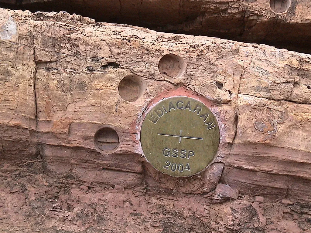
• The Ediacaran, base defined at Enorama Creek, Flinders Ranges, South Australia, ratified on 12 March 2004. Its golden spike sits at the bottom of a distinctive “cap carbonate” (the Nuccaleena Formation) laid directly over the debris of a global glaciation. It was the first internationally ratified new period in over 120 years.
• The Cambrian, base defined at Fortune Head, Newfoundland, where the boundary is drawn on a trace fossil rather than a body fossil: Treptichnus pedum, the burrow of an animal nobody has ever seen, whose complex branching burrows provide a correlatable marker close to the early diversification of bilaterian-style behaviour.
• The Cretaceous–Paleogene boundary, defined at El Kef, Tunisia, at the base of the boundary clay at El Kef; the associated iridium anomaly is one of the principal signals used to correlate the boundary globally.
• The Holocene, our own epoch, whose base is defined not in rock at all but in ice: a specific depth (1492.45 m) in the NGRIP ice core from Greenland, dated to 11,700 years before the year 2000.
• The Meghalayan, the age we currently live in, defined in a stalagmite from Mawmluh Cave in northeast India, marking a roughly 200-year drought recorded on several continents that struck about 4,250 years ago.

Not everything has a golden spike. Most Precambrian boundaries are GSSAs, Global Standard Stratigraphic Ages, defined by round-number dates rather than physical points. Much of the Precambrian lacks the abundant, rapidly evolving and widely distributed fossil assemblages that make high-resolution Phanerozoic biostratigraphy possible. When you cannot find a natural marker in the rock, you fall back on a number. The base of the Proterozoic is set at 2.5 billion years, a round number chosen by committee. The base of the Archean was a round 4.0 billion until the ICS tied it to the oldest known rock, the Acasta Gneiss, at 4,031 ± 3 million years, and in 2022 ratified a Hadean GSSA at 4,567.30 ± 0.16 Ma, based on the age of the oldest dated Solar-System solids. For these earliest intervals, the ICS has instead adopted chronometric reference ages tied to exceptionally old terrestrial rocks or Solar-System material.

The tour up the scale

Now we walk up the whole thing, oldest to youngest, with dates from the current ICS chart, what defines each base, the events that matter, and where each name came from. Alongside runs a second scale: all 4.54 billion years compressed into one calendar year (the arithmetic is at the end).

Hadean (4.567 to 4.031 billion years ago)

The Hadean is named for Hades, and it earned it. This is the eon of formation: a planet assembling from the protoplanetary disk, undergoing differentiation, magma-ocean episodes and major impacts, and the collision with a Mars-sized body that threw off the debris that became the Moon. There are no Hadean rocks to speak of, only those stubborn Jack Hills zircons, surviving in younger rock, whispering that liquid water and a solid crust existed astonishingly early. On the calendar year, the Hadean runs to about 10 February on this calendar. Earth spends the first six weeks of its year molten, bombarded, and only slowly acquiring a crust.

Archean (4.031 to 2.5 billion years ago)

The Archean gives us the first stable crust, the first oceans, and some of the earliest widely accepted evidence for life. By around 3.5 billion years ago, shallow seas held stromatolites: layered mounds built by mats of photosynthesising microbes. They are among the oldest widely accepted evidence for life on Earth, and living versions still grow today in places like Shark Bay, Western Australia. Life at this point is single-celled, and the air is unbreathable, essentially no free oxygen.

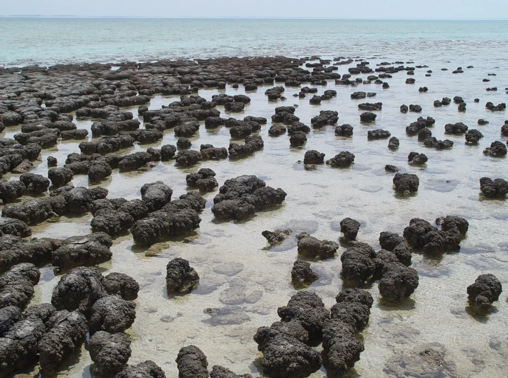
The Archean crust also records the planet’s oldest scars. Geoscopy’s own coverage of the Pilbara’s ancient impact structure and the giant Vredefort event shows how much of the early record is written in shattered rock. On the calendar, from mid-February to mid-June (the 2.5-billion-year mark falls on 13 June). Life appears in late March; for months, the year’s only inhabitants are microbes.

Proterozoic (2.5 billion to 538.8 million years ago)

The Proterozoic is the longest eon, and three of its events reshaped the planet. First, the Great Oxidation Event, around 2.4 to 2.3 billion years ago: cyanobacteria had been making oxygen for a while, but now it began to accumulate in the atmosphere for the first time. To most existing life, oxygen was a poison; the GOE was probably the first great extinction, invisible because it killed things too small to fossilise well. Its signature is written in the rocks as banded iron formations, spectacular striped deposits of iron oxide, precipitated as newly available oxygen rusted the iron dissolved in the ancient oceans.

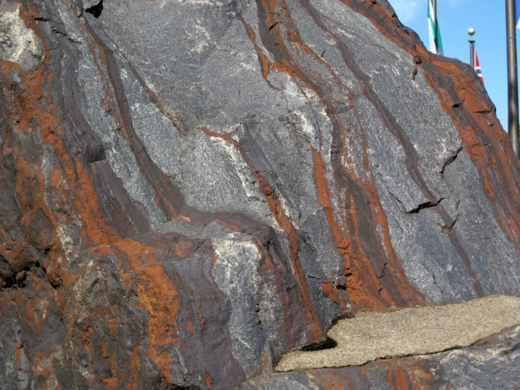
Second, the Snowball Earth glaciations of the Cryogenian Period, roughly 720 to 635 million years ago, when ice may have reached the equator and ice extended to low latitudes and perhaps close to the equator; how completely sea ice covered the global ocean remains debated. Geoscopy covers the evidence for these global freezes and the return of banded iron formations that accompanied them in its dedicated Snowball Earth and banded iron pieces. Third, in the twilight of the eon, the Ediacaran biota, the first widespread assemblages of large, complex, soft-bodied organisms, strange fronds and discs like Dickinsonia, living on the seafloor largely before skeletons or predators existed (the first mineralised tubes, and the first bore-holes in them, appear only at the very end of the Ediacaran).

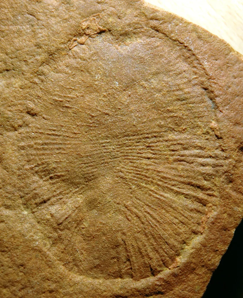
On the calendar year, the Proterozoic runs from 13 June to 18 November. Oxygen begins to accumulate around the solstice, on 21 June; the Snowball glaciations bite in early November; in the final week before the explosion. Everything before this, 88% of Earth’s history, is the Precambrian, an informal catch-all for the three eons before the Cambrian. “Precambrian” is an informal collective term for the Hadean, Archean and Proterozoic rather than a formal eon of its own.

Paleozoic Era: the Cambrian (538.8 to 486.85 million years ago)

The Phanerozoic Eon, “visible life”, begins with the Cambrian radiation. The Cambrian explosion is the geologically sudden appearance, over a few tens of millions of years, of many major animal lineages became conspicuous in the fossil record, alongside a rapid expansion of skeletonised forms and ecological complexity: arthropods, molluscs, the first chordates, animals with eyes, limbs, guts and armour. The base of the Cambrian, and therefore of the entire Phanerozoic, is that Treptichnus pedum burrow at Fortune Head. The showcase is the Burgess Shale of British Columbia, where soft bodies were fossilised in exquisite detail around 508 million years ago: the half-metre predator Anomalocaris, the five-eyed Opabinia, the spiny Hallucigenia, and Marrella, the “lace crab” that fits into no living arthropod group.

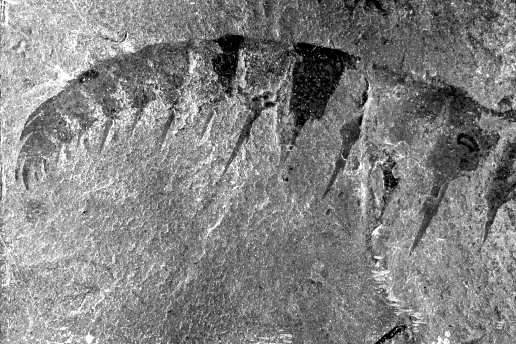
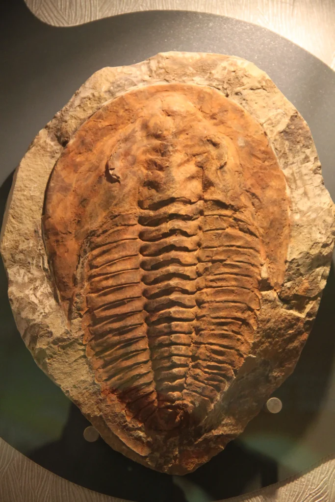
The Cambrian also gives us the trilobites, the emblematic arthropods that scuttle through the entire Paleozoic. On the calendar, the Cambrian begins around 18 November. Everything you think of as “the age of animals” is crammed into the last six weeks of the year.

Ordovician (486.85 to 443.1 million years ago)

Lapworth’s compromise period, the Ordovician, saw life diversify enormously in the sea and the first tentative move of plants onto land. It ended in catastrophe: the end-Ordovician mass extinction, which eliminated roughly half of all marine genera and nearly 85% of marine species as the planet plunged into a sharp glaciation, ranking it as the second-largest of the “Big Five.” This is also the period tied to the intriguing hypothesis that Earth briefly had a ring system, explored in Geoscopy’s coverage of the idea.

Silurian (443.1 to 419.6 million years ago)

Murchison’s period is short but pivotal: life established itself firmly on land. The first vascular plants spread across the continents, and the first unambiguous land animals, arthropods, followed. Coral reefs flourished in warm shallow seas. The Silurian is the quiet, green interval between two more dramatic neighbours.

Devonian (419.6 to 358.9 million years ago)

Call it the Age of Fishes. The Devonian seas teemed with armoured giants like Dunkleosteus, and it was here that lobe-finned fish began hauling themselves onto land, the lineage that leads, eventually, to us, with Tiktaalik as the celebrated intermediate. On land, the first true forests appeared, and with them the first deep, root-bound soils. The period closed with the Late Devonian extinction, a drawn-out series of pulses that hit reef ecosystems especially hard.

Carboniferous (358.9 to 298.9 million years ago)

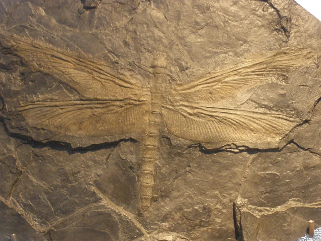
The Carboniferous is named for its extensive coal-bearing strata, and its tropical wetlands produced many of the great coal seams later mined in Europe and North America. Vast swampy forests of giant club-mosses and ferns whose buried remains became the coal seams that later powered the Industrial Revolution. Atmospheric oxygen rose to perhaps 35%, well above today’s 21%, and in that oxygen-rich air arthropods grew monstrous: dragonfly-like Meganeura with wingspans near 70 centimetres, and millipedes over two metres long. The Carboniferous is the one period the ICS formally splits in two: the Mississippian and the Pennsylvanian, names that began as North American units and now sit on the international chart as sub-periods.

Permian (298.9 to 251.9 million years ago)

The continents fused into the single supercontinent Pangaea, and the Paleozoic ended in the worst catastrophe life has ever faced: the end-Permian extinction, the “Great Dying,” 251.9 million years ago. Driven by the vast volcanic eruptions of the Siberian Traps, whose greenhouse-gas emissions drove rapid warming and contributed to ocean acidification and widespread deoxygenation, it killed, in the words of a 2015 MIT News report on the Siberian Traps, ‘more than 96 percent of marine species and 70 percent of land species’ (more recent tallies put marine species loss nearer 80 per cent). Life very nearly ended entirely. Geoscopy covers this in depth in The Great Dying, and the assembly and future of supercontinents in Pangaea Ultima. This extinction is the boundary John Phillips drew, blind, in 1841: the line between Paleozoic and Mesozoic.

Mesozoic Era: Triassic (251.9 to 201.4 million years ago)

Recovery from the end-Permian extinction was slow and uneven. In the recovery world of the Triassic, the survivors radiated into new forms, and among them appeared the first dinosaurs, the first mammals, and the first flying reptiles. The period ended with another mass extinction, the fourth of the Big Five, which cleared ecological space and let the dinosaurs take over.

Jurassic (201.4 to 143.1 million years ago)

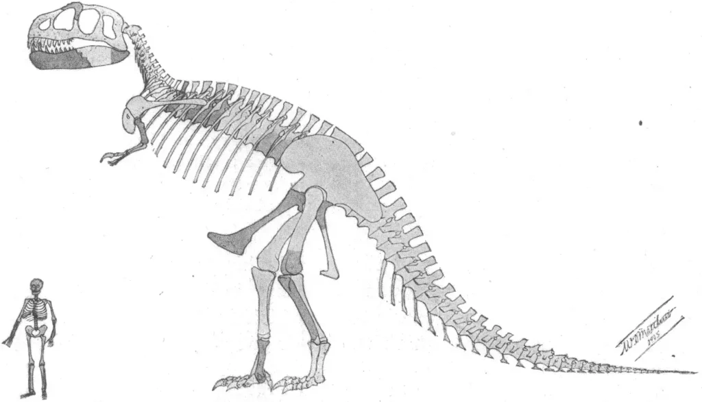
The age of giant dinosaurs proper. Long-necked sauropods, the largest animals ever to walk the Earth, browsed forests of conifers and cycads; the first birds, like Archaeopteryx, took to the air. Named for the Jura Mountains, the Jurassic is warm, green, and dominated by reptiles on land, in the sea, and in the sky.

Cretaceous (143.1 to 66.0 million years ago, and the base still awaits a golden spike)

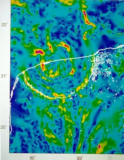
The longest period of the Mesozoic, the Cretaceous saw flowering plants appear and spread, remaking terrestrial ecosystems. And then, 66 million years ago, it ended in the most famous boundary in all of geology. An asteroid roughly ten kilometres across struck what is now the Yucatán Peninsula, blasting out the buried Chicxulub crater and throwing enough debris into the atmosphere to darken the planet. Around three-quarters of species died, including every non-avian dinosaur. The evidence is that iridium-rich clay layer, found worldwide and defined at El Kef, and, at the Tanis site in North Dakota, the debris of the impact’s first hours appears to be preserved. Geoscopy also covers a smaller, later impact in the Silverpit crater of the North Sea. On the calendar year, the dinosaurs die on about 26 December.

Cenozoic Era: Paleogene (66 to 23.04 million years ago)

The K–Pg extinction opened ecological niches on land and in the oceans, and mammals diversified rapidly during the Paleogene.; the Age of Mammals had begun. The Paleogene (Paleocene, Eocene, Oligocene epochs) saw mammals grow from small survivors into the ancestors of whales, horses, primates and the rest. Climates were warm early on, then cooled toward the first Antarctic ice.

Neogene (23.04 to 2.58 million years ago)

Grasslands spread; grazing mammals and our own ape ancestors diversified. Late in the Neogene came one of the strangest events in the geologic record: the Messinian Salinity Crisis, between 5.96 and 5.33 million years ago, when the Mediterranean was cut off from the Atlantic and very nearly dried up, leaving kilometre-thick beds of salt and gypsum across its floor. Geoscopy tells the full story in its account of the Mediterranean’s disappearance.

Quaternary (2.58 million years ago to now)

Our period. The Quaternary is the age of ice ages, repeated advances and retreats of great ice sheets across the Northern Hemisphere, and of humans. Its first epoch, the Pleistocene, is the classic Ice Age of mammoths and Neanderthals; sea levels rose and fell by more than a hundred metres, exposing and drowning land bridges like Doggerland beneath what is now the North Sea. The magnetic reversals and excursions of this interval, including the Laschamps event, are recorded in Quaternary rocks and ice.

The Holocene, the current epoch, began 11,700 years ago as the last ice age released its grip, and it is the epoch of human civilisation, agriculture and cities. In 2018 the ICS formally subdivided it into three ages: the Greenlandian (11,700 to 8,200 years ago), the Northgrippian (8,200 to 4,200 years ago), and the Meghalayan (4,200 years ago to today). We live in the Meghalayan. On the calendar year, our species appears at roughly 11:25 pm on 31 December, and all of recorded human history, every pyramid, empire, and equation, occupies the final 35 seconds before midnight.

Why the scale is so lopsided, and the names such a mess

Look again at the chart. The Precambrian (Hadean, Archean and Proterozoic together) is nearly 88% of Earth’s history, and on most charts it gets a thin band at the bottom. The Phanerozoic, a mere 12% of time, gets subdivided into dozens of finely drawn periods, epochs and ages. Why the distortion?

The answer is fossils. Chronological resolution comes from biological change, and abundant, hard-shelled, fast-evolving fossils only exist from the Cambrian onward. In the Phanerozoic, faunas turn over fast enough to slice time thinly and correlate rocks worldwide. In the Precambrian, with almost nothing but microbes for three billion years, there is simply nothing to subdivide it with, hence the round-number GSSAs and the vast, sparsely labelled expanses. The distortion follows the evidence.

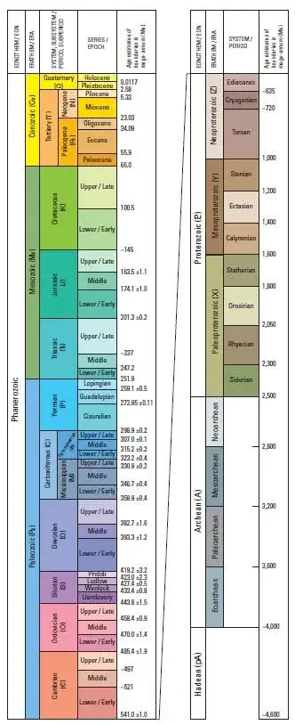
The names are a mess for a different reason: history. The scale was assembled piecemeal over two centuries by rival geologists naming things after Welsh tribes (Ordovician, Silurian), English counties, Russian provinces (Permian), and rock types (Cretaceous, from the Latin for chalk; Carboniferous, “coal-bearing”). It grew by accretion over two centuries.

Two renamings matter. First, “Tertiary” was retired. For most of the scale’s history the Cenozoic was split into Tertiary and Quaternary; the ICS replaced “Tertiary” with the cleaner pair Paleogene and Neogene to match the rest of the chart. Second, and more dramatically, the Quaternary was nearly abolished in the process, swallowed into the Neogene, before an outcry from geologists who study the ice ages and human origins. They pointed out that the Quaternary marks a genuine, distinctive interval, and on 29 June 2009 the IUGS formally reinstated it as a full period with its base fixed at 2.58 million years ago. The now-familiar three-period Cenozoic (Paleogene, Neogene, Quaternary) dates only from that 2009 decision.

The Anthropocene: the case, the vote, and why we still live in the Holocene

You have almost certainly heard that we live in the “Anthropocene”, the age of human impact. In everyday usage, yes. On the official chart, no, and the vote that settled it is the newest chapter in the scale’s history.

The term was popularised around 2000 by Paul Crutzen and Eugene Stoermer. In 2009 the ICS set up an Anthropocene Working Group to test whether human impact had left a signal in the rock sharp enough to define a new epoch. After fifteen years, the group proposed a start date of the 1950s, the “Great Acceleration”, with a golden spike in the sediments of Crawford Lake, Canada, marked by plutonium fallout from nuclear tests, fly ash and microplastics.

The Subcommission on Quaternary Stratigraphy (SQS) voted over the preceding month, and the result was released on 4 March 2024, whose 18 members required a 60% supermajority for approval. It was rejected by 12 votes (66%) against, 4 in favour, with 2 abstentions. The decision was upheld by the ICS and formally ratified by the IUGS on 20 March 2024. The objections were largely stratigraphic: many geologists felt that compressing an epoch into a mere seventy years, barely a human lifetime, against periods measured in tens of millions of years, misused the machinery of the time scale, and that a proposed boundary in the 1950s ignored the far older and more profound human transformation of the planet through agriculture and land clearance.

So, officially, we still live in the Holocene, in the Meghalayan Age. The rejection did not deny that humans are reshaping the Earth; the IUGS statement itself expects the term to stay in use, and many geologists prefer to treat the Anthropocene as an ongoing event, like the Great Oxidation Event, rather than a bounded unit. The signal is in the sediment. What the committee declined was the spike.

The time scale as a working tool

The time scale is the single most useful correlation tool in the Earth sciences. Because fossils appear in the same order everywhere, a geologist can pick up a rock in Texas, identify its fossils or its ash-bed date, and know precisely which layer to look for in Nigeria or China. That is how petroleum and mining geologists find what they are looking for: oil, coal, and ore bodies form in specific intervals of time, and correlating strata across continents is how you predict where they lie. An oil geologist who can say “this is a Late Jurassic source rock” is making a multimillion-dollar prediction grounded entirely in the time scale. Geoscopy’s guide to rock identification is the practical starting point for reading those layers yourself.

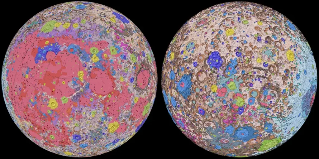
The idea travels beyond Earth, too. The Moon has its own geologic time scale, the Pre-Nectarian, Nectarian, Imbrian, Eratosthenian and Copernican periods, built not from fossils, which it lacks, but from impact craters and the debris blankets they throw out. Mars has one as well. Where there are no fossils, geologists date surfaces by counting craters, but the principle is identical: use the physical record to put events in order and then hang numbers on them.

The clock, done properly

Now the calendar year, computed from scratch. The assumption is simple: squeeze 4.54 billion years into 365.25 days.

Dividing, one day equals 4.54 billion ÷ 365.25 = about 12.43 million years. From there: one hour ≈ 518,000 years; one minute ≈ 8,600 years; one second ≈ 144 years. Now place the markers, each computed as time-before-present converted to days and counted back from midnight on 31 December:

• Formation of the Earth: 1 January, 00:00.
• First life (stromatolites, ~3.5 Ga): 3,500 ÷ 12.43 = 282 days before year-end → late March.
• Great Oxidation Event (~2.4 Ga): 193 days before year-end → around 21 June. The air does not start becoming breathable until midsummer.
• Cambrian explosion (538.8 Ma): 538.8 ÷ 12.43 = 43.3 days before year-end → about 18 November. Complex animals wait until the year’s final six weeks.
• Non-avian dinosaurs die (66 Ma): 66 ÷ 12.43 = 5.3 days before year-end → about 26 December.
• Homo sapiens appears (~300 ka): 300,000 ÷ 144 ≈ 2,080 seconds ≈ 35 minutes before midnight → roughly 11:25 pm on 31 December.
• All recorded history (~5,000 years): 5,000 ÷ 144 ≈ 35 seconds before midnight.

Run the same exercise on a 24-hour clock, and it is starker still. Our species, at 300,000 years out of 4.54 billion, appears just under 6 seconds before midnight. Every human who has ever lived, every word ever written, occupies the last blink of the geological day.

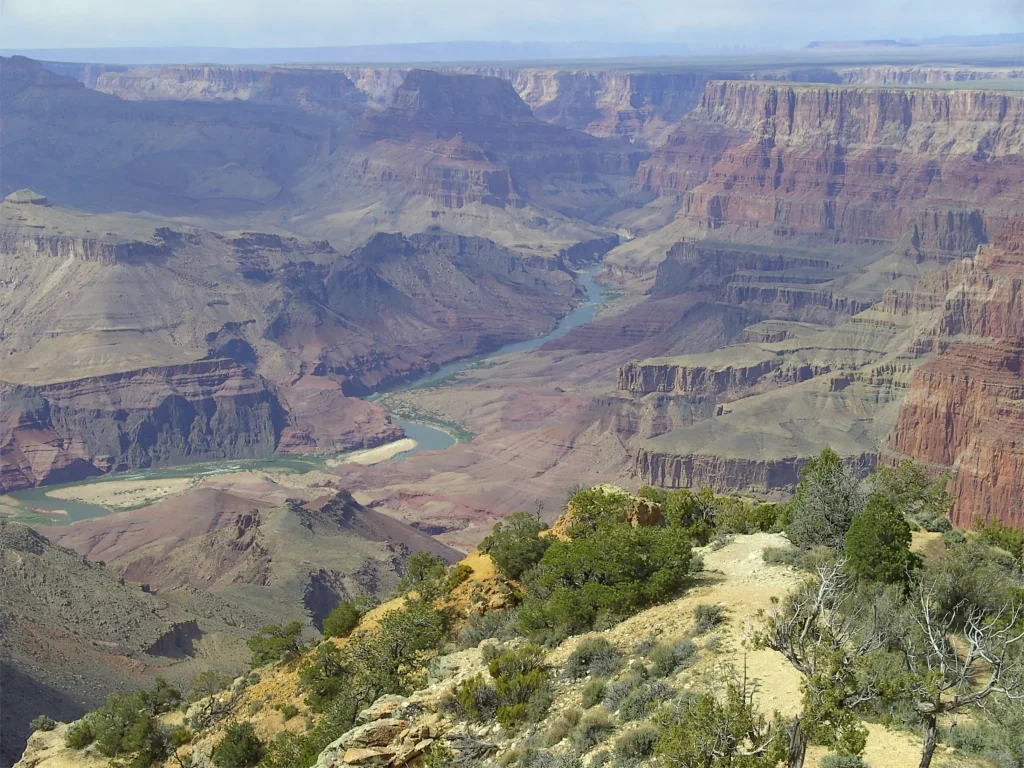
Stand at Siccar Point today and you can put your hand flat on Hutton’s unconformity, one palm on Silurian rock, the other on Devonian, with tens of millions of years of vanished time running between your fingers. The whole geologic time scale is the dated, golden-spiked version of that one touch.

Frequently Asked Questions

What are the four eons of geologic time?

From oldest to youngest, the four eons are the Hadean (4.567 to 4.031 billion years ago), the Archean (4.031 to 2.5 billion years ago), the Proterozoic (2.5 billion to 538.8 million years ago) and the Phanerozoic (538.8 million years ago to today). The first three together are informally called the Precambrian, which covers roughly 88% of Earth’s history.

What era, period and epoch are we in right now?

We live in the Phanerozoic Eon, the Cenozoic Era, the Quaternary Period, the Holocene Epoch and, since a 2018 ICS decision, the Meghalayan Age. Despite popular usage, the Anthropocene is not an official epoch; a 2024 vote kept us formally in the Holocene.

How is the geologic time scale divided?

It is a nested hierarchy: eons contain eras, eras contain periods, periods contain epochs, and epochs contain ages. Each unit has a “rock” twin (system, series, stage) for the physical strata. The International Commission on Stratigraphy maintains the divisions and publishes the official chart.

Why is the Precambrian so long?

The Precambrian spans nearly four billion years because life stayed simple and microscopic for most of it. Chronological resolution comes from fossils, and abundant hard-shelled fossils only appear from the Cambrian onward, so there is little biological change to subdivide the earlier eons, hence their vast, sparsely labelled expanses.

How do geologists know how old a rock is?

Two main methods. Relative dating uses superposition (lower layers are older) and index fossils to order rocks. Absolute dating uses radioactivity: unstable atoms decay to stable ones at a fixed rate, so measuring parent and daughter atoms in a mineral such as zircon gives a numerical age. Uranium-lead and argon-argon dating are the standard techniques.

How do we know the Earth is 4.54 billion years old?

Clair Patterson measured the lead isotopes in the Canyon Diablo meteorite in 1956 and calculated 4.55 billion years, plus or minus about 70 million. Meteorites formed at the same time as the planets, so they date the whole solar system. Decades of further measurements have refined the figure to 4.54 billion years.

What is a golden spike?

A golden spike, formally a Global Boundary Stratotype Section and Point (GSSP), is a single physical point in a specific rock outcrop that defines a time boundary by international agreement. The boundary is the rock, not a date, so the date can be revised without moving the definition. Examples include Fortune Head (base of the Cambrian) and El Kef (the Cretaceous–Paleogene boundary).

What is the Cambrian explosion?

The Cambrian explosion is the geologically rapid appearance, starting about 538.8 million years ago, of nearly all major animal body plans, arthropods, molluscs, chordates and more. The Burgess Shale of Canada preserves this burst of life in extraordinary soft-bodied detail, including the predator Anomalocaris.

Is the Anthropocene an official epoch?

No. On 4 March 2024 the Subcommission on Quaternary Stratigraphy voted 12 to 4 (with 2 abstentions) against formalising the Anthropocene, and the IUGS upheld the decision on 20 March 2024. We officially remain in the Holocene. Geologists increasingly treat “Anthropocene” as an ongoing event rather than a formal unit of the time scale.

What is the difference between the geologic and the geological time scale?

There is no scientific difference. “Geologic time scale” is the more common American spelling and “geological time scale” the standard British form. Both refer to the same ICS-maintained framework of eons, eras, periods and epochs.

Summary chart: eons, eras and periods with ICS dates

Eon	Era	Period	Began (Ma unless noted)	Defining event / base
Phanerozoic	Cenozoic	Quaternary	2.58	Onset of Northern Hemisphere ice ages
Phanerozoic	Cenozoic	Neogene	23.03	Grasslands spread; Messinian Salinity Crisis late in period
Phanerozoic	Cenozoic	Paleogene	66.0	Base at the K–Pg iridium layer (El Kef, Tunisia)
Phanerozoic	Mesozoic	Cretaceous	~145	Ends with Chicxulub impact, 66 Ma
Phanerozoic	Mesozoic	Jurassic	201.4	Age of giant dinosaurs; first birds
Phanerozoic	Mesozoic	Triassic	251.9	Recovery after the Great Dying; first dinosaurs
Phanerozoic	Paleozoic	Permian	298.9	Pangaea; ends in end-Permian extinction, 251.9 Ma
Phanerozoic	Paleozoic	Carboniferous	358.86	Coal forests; ~35% oxygen; giant insects
Phanerozoic	Paleozoic	Devonian	419.2	Age of Fishes; first forests
Phanerozoic	Paleozoic	Silurian	443.1	Life colonises the land
Phanerozoic	Paleozoic	Ordovician	486.85	Ends in second-largest mass extinction
Phanerozoic	Paleozoic	Cambrian	538.8	Base on Treptichnus pedum (Fortune Head); Cambrian explosion
Proterozoic	—	(Ediacaran to Siderian)	2500	Great Oxidation Event; Snowball Earth; Ediacaran biota
Archean	—	—	4031	First crust, oceans, and life (stromatolites)
Hadean	—	—	~4567	Planet forms; Moon-forming impact