Introduction

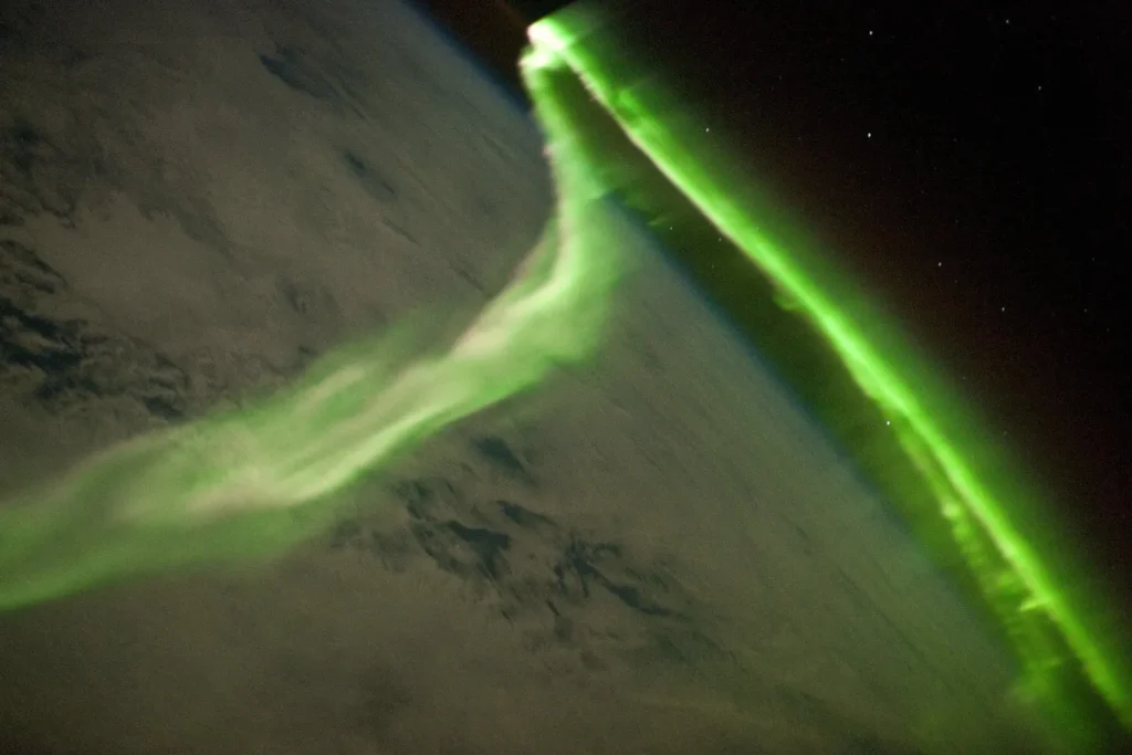
In a fourth-floor office of the Climate and Space Sciences and Engineering Department at the University of Michigan, Agnit Mukhopadhyay is watching a planet he does not entirely recognize. On his monitor, a three-dimensional reconstruction of Earth’s magnetosphere from 41,000 years ago is running on the Space Weather Modeling Framework. The auroral oval, the ring of charged-particle precipitation that today brushes Tromsø and Yellowknife, has detached from the pole. It is sliding south. Spain glows. Northern Egypt glows. The shape of the ring is wrong: not a ring at all but a sprawling, multi-lobed bruise across the upper atmosphere.

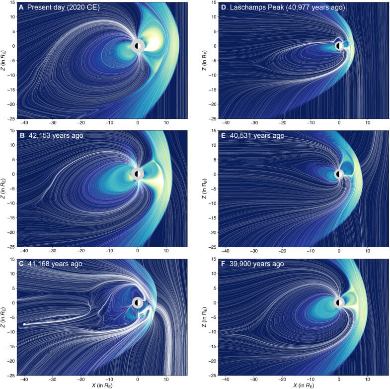
Mukhopadhyay’s simulation, published in Science Advances on 16 April 2025, shows what happened during the Laschamps geomagnetic excursion, when Earth’s dipole field shrank to roughly 10 percent of its present strength and the magnetic poles wandered toward the equator. “What surprised me most was how profoundly the auroral dynamics changed,” he told the European Geosciences Union’s Solar-Terrestrial Sciences division in July 2025. “In our simulations, auroral precipitation wasn’t limited to the familiar high-latitude oval structures of today’s dipole-dominated magnetosphere.”

Earth carries the memory of a magnetic catastrophe in lava, ice, and tree rings. The latest satellite data shows a slice of that catastrophe stirring again beneath the South Atlantic.

What Happened 41,000 Years Ago

The story begins, by accident, with a roadcut. In the early 1960s, Norbert Bonhommet, then at the Institut de Physique du Globe de Strasbourg, was sampling lava flows in the Chaîne des Puys, a chain of cinder cones in France’s Massif Central. He was sampling for a paleomagnetic record of late Quaternary lavas. He found something else. At the village of Laschamps, and again at neighboring Olby, the magnetite grains in the basalt were pointing the wrong way. North was south. South was north.

Bonhommet and his colleague J. Babkine published the result in 1967 in a short note to the Comptes Rendus de l’Académie des Sciences. For a while it was taken as evidence of a true geomagnetic reversal, the youngest yet known. Skeptics later argued it was a chemical artifact of self-reversing minerals, and the question hung unresolved through the 1980s, until paleointensity measurements at Laschamps and Louchadière showed field strengths of roughly 8 microteslas, about a fifth of today’s local field confirming a real geomagnetic event. The “Laschamps excursion” entered the literature: a brief, deep weakening of Earth’s dipole, dated by argon-argon and radiocarbon methods to about 41,000 years ago, with the most acute phase now placed between 42,200 and 41,500 years before present.

It is now the most thoroughly documented magnetic excursion in the geological record. Cosmogenic radionuclides, atoms produced when galactic cosmic rays smash into nitrogen and oxygen in the upper atmosphere, preserve the signature in Greenland and Antarctic ice cores. The average production rate of beryllium-10 during the Laschamps excursion was two times higher than present-day production, according to Sanja Panovska’s reconstruction. Carbon-14 production spiked. The shield was down.

At the European Geosciences Union General Assembly in Vienna on 19 April 2024, Panovska, a geomagnetism researcher at the GFZ Helmholtz Centre for Geosciences in Potsdam, presented a reconstruction combining paleomagnetic data with cosmogenic-isotope records (abstract EGU24-10977). Her model resolves the excursion into distinct phases. The transition from normal to reversed polarity took about 250 years; the field then sat in its reversed configuration for roughly 440 more. During the transition itself, when the dipole was collapsing, the global field dropped to as little as 5 percent of modern intensity. While fully reversed, it recovered to roughly 25 percent. (These specific numerical phase estimates appear in Panovska’s EGU presentation and in EurekAlert!-syndicated coverage rather than in a stand-alone peer-reviewed paper, and should be read with that caveat.)

“Understanding these extreme events is important for their occurrence in the future, space climate predictions, and assessing the effects on the environment and on the Earth system,” Panovska said in the EurekAlert! release accompanying her talk.

The Mukhopadhyay et al. paper, on which Panovska is second author, uses a similar reconstruction as the inner boundary condition for the magnetosphere itself. Their headline figure: a magnetosphere that did not so much shield Earth as drape it. The bow shock contracted. Open field lines, the channels along which solar wind plasma can reach the ionosphere, spread across mid-latitudes. The aurora, normally pinned to the polar caps, sprawled. For about three centuries, the planet’s space environment resembled that of Uranus or Neptune rather than today’s orderly dipole.

The Kauri Tree That Changed the Story

In 2019, peat workers near Ngāwhā, in New Zealand’s Northland Region, hauled a 60-tonne Agathis australis, a swamp kauri, out of a bog. Radiocarbon dating put the tree’s growing years between roughly 42,500 and 41,000 years ago. Its rings spanned the Laschamps excursion in annual resolution.

That tree became the centerpiece of a paper by Alan Cooper, then of the South Australian Museum, and Chris Turney of UNSW Sydney, published in Science on 19 February 2021. Cooper and Turney’s team used the kauri’s carbon-14 spike to anchor a global chronology and then layered onto it a model of atmospheric chemistry, climate, and human behavior during the field collapse. They concluded that the geomagnetic minimum drove ozone depletion, mid-latitude UV-B increase, climate reorganization, and most provocatively a cascade of biological and cultural changes: Australian megafaunal extinctions, the disappearance of Neanderthals in Eurasia, the eruption of figurative cave art across Europe and Sulawesi.

They named the most acute phase of the collapse the “Adams Transitional Geomagnetic Event,” after Douglas Adams, whose Hitchhiker’s Guide to the Galaxy had famously declared 42 to be the answer to life, the universe, and everything. “The more we looked at the data, the more everything pointed to 42,” Turney told reporters. “It was uncanny. Douglas Adams was clearly on to something, after all.”

“Early humans around the world would have seen amazing auroras, shimmering veils and sheets across the sky,” Cooper said in a UNSW Sydney press release accompanying the paper. The team’s modelled scenario put the planet briefly under a magnetic field as low as a few percent of modern, with cave art emerging as a behavioral response to a harsher UV environment outside.

The paper landed like a stone in a small pond.

The Counterattack

Within nine months, two formal Technical Comments appeared in Science. The first, led by Andrea Picin of the Max Planck Institute for Evolutionary Anthropology and including Chris Stringer of the Natural History Museum in London and Jean-Jacques Hublin, attacked the chronology. Neanderthal disappearance, the Picin group argued, was a process distributed across thousands of years and several glacial stadials, not a pulse at 42 kya. Australian megafaunal collapse was not synchronously dated to that horizon either. And the behavioral markers Cooper and Turney attributed to UV stress, cave use, ochre, tailored clothing, were already established in Borneo, Sulawesi, and possibly Europe tens of thousands of years before the Laschamps minimum.

“All in all, not only have Cooper and colleagues failed to provide convincing explanatory mechanisms relating the Laschamps excursion to cultural and biological changes,” Picin and his coauthors wrote, “but their chronological coincidence with this geomagnetic reversal is highly questionable.”

The second comment, from the paleoanthropologist John Hawks of the University of Wisconsin–Madison, was more pointed still. Hawks reread every citation Cooper and Turney had used to anchor extinctions and bottlenecks to the 42,000-year mark. He found, in case after case, that the cited papers either gave wider confidence intervals, different point estimates, or modes of statistical distributions that had been read as discrete events. The thylacine bottleneck cited at “around 42 ka” was, in the original source, dated to 20,400 years before present.

“Any reader of Douglas Adams should understand that the importance of ’42’ is that no one knows what the question is.”

John Hawks, Science, 2021

Cooper and Turney responded in the same issue, holding to their hypothesis and arguing that recalibration of the radiocarbon curve had moved many events closer to the Laschamps horizon. The exchange did not produce consensus. Most archaeologists and paleogeneticists working on the late Pleistocene now treat the strong Cooper-Turney claims, Neanderthal extinction caused by ultraviolet light, megafaunal extinctions triggered by a magnetic event, as not established.

There is a useful skeptical control in the geological record. The Blake excursion, about 125,000 years ago, involved comparable or even longer-duration dipole weakening. The deviation lasted roughly 6,500 years, according to sediment cores from the Blake–Bahama Outer Ridge in the North Atlantic. The Blake event left no detectable global extinction pulse, no documented cultural transition, no preserved spike of cave use. If geomagnetic excursions reliably drove biological catastrophe, the Blake excursion should have produced one. It did not.

That does not mean the Laschamps was inert. It means the human-evolution argument is a long way from being the right story.

Auroras at the Equator

Mukhopadhyay’s group set out to model the physics of the excursion without making strong claims about its biological consequences. They folded three pieces together: Panovska’s paleomagnetic-cosmogenic reconstruction of the global field during the excursion (LSMOD.2); the Space Weather Modeling Framework, originally built to simulate solar storms striking the modern magnetosphere; and a model of ionospheric and atmospheric response.

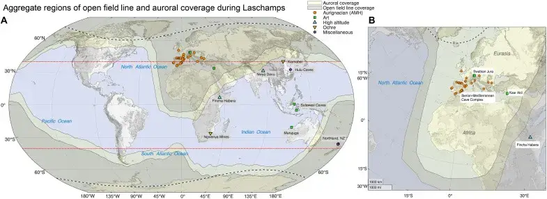
The result is the first three-dimensional reconstruction of Earth’s geospace during a geomagnetic excursion. The numbers are striking. The dayside magnetopause, the boundary at which solar wind pressure balances the planet’s magnetic pressure, contracted from roughly 10 Earth radii to as little as 3 or 4 in some configurations. Open field lines, normally restricted to polar caps, threaded down to subtropical latitudes. The team coined the term “global aurora” or “omni-aurora” for what their simulations produced: auroral precipitation not as a ring but as a sprawling, time-varying patchwork stretching across most of the globe.

“In the study, we combined all of the regions where the magnetic field would not have been connected, allowing cosmic radiation, or any kind of energetic particles from the sun, to seep all the way in to the ground,” Mukhopadhyay said in the University of Michigan press release on 16 April 2025. “We found that many of those regions actually match pretty closely with early human activity from 41,000 years ago, specifically an increase in the use of caves and an increase in the use of prehistoric sunscreen.”

The “sunscreen”, red ochre, ground from iron-rich earths and rubbed on skin, is a real ethnographic and archaeological category, and a real UV blocker. Mukhopadhyay’s coauthor Raven Garvey, an anthropologist at Michigan, was careful with the inference. “I think it’s important to note that these findings are correlational and (ours is a) meta analysis, if you will,” she said in the same release. “But I think it is a fresh perspective on these data in light of the Laschamps excursion.”

Whether or not the ochre-and-caves correlation survives further work, the geophysical result stands on its own. For a few centuries, Earth’s magnetosphere behaved like that of an outer planet. The familiar architecture, a tight dipole, a polar auroral oval, a sharp distinction between trapped radiation belts and open atmosphere, fell apart and reassembled.

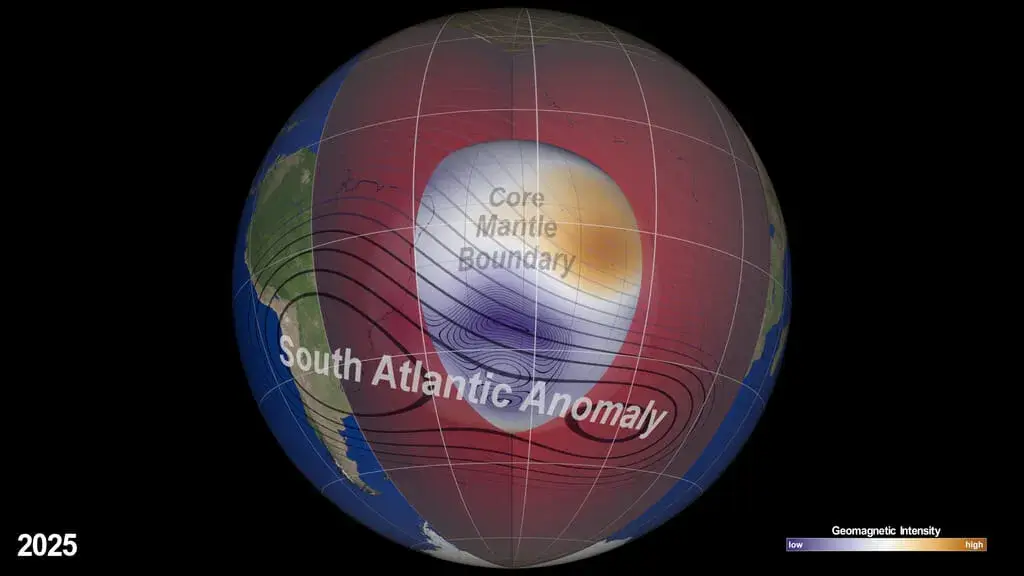
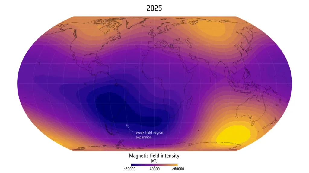
The South Atlantic Anomaly: A Whisper, Not a Siren

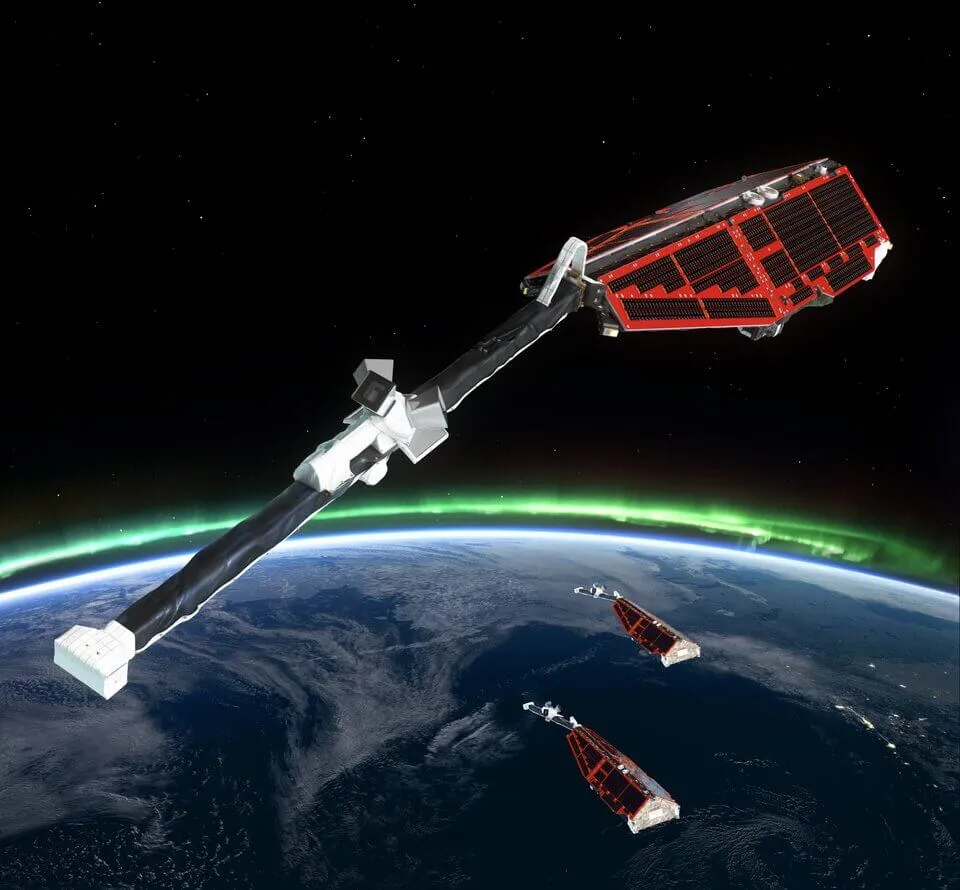
Now to October 2025. The European Space Agency’s Swarm constellation, three identical satellites launched on 22 November 2013 into low Earth orbit, each carrying a vector magnetometer and an absolute scalar magnetometer, has now produced the longest continuous space-based record of Earth’s main magnetic field. In September 2025, Chris Finlay, professor of geomagnetism at DTU Space at the Technical University of Denmark, and his colleagues Clemens Kloss and Nicolas Gillet published the eleven-year model in Physics of the Earth and Planetary Interiors (DOI: 10.1016/j.pepi.2025.107447).

The headline result, announced by ESA on 13 October 2025: the South Atlantic Anomaly has grown by an area nearly half the size of continental Europe since Swarm’s launch: an expansion equal to 0.9 percent of Earth’s surface area. The anomaly is not weakening uniformly. A patch of ocean southwest of Africa has been losing field strength faster than the rest since 2020, and the anomaly is splitting into two distinct cells. Inside the cells, satellite electronics are taking hits.

“The South Atlantic Anomaly is not just a single block,” Finlay said in the ESA release. “It’s changing differently towards Africa than it is near South America. There’s something special happening in this region that is causing the field to weaken in a more intense way.”

That “something special” is visible when the Swarm team projects the surface field downward to the core-mantle boundary, the seam at roughly 2,900 kilometers depth where Earth’s mantle meets its molten outer core. There, beneath the South Atlantic and southern Africa, sit patches of reversed-polarity flux: regions where field lines, instead of emerging from the core into the southern hemisphere as a normal dipole would predict, plunge back into it.

“Normally we’d expect to see magnetic field lines coming out of the core in the southern hemisphere. But beneath the South Atlantic Anomaly we see unexpected areas where the magnetic field, instead of coming out of the core, goes back into the core.”

Chris Finlay, DTU Space

These reversed flux patches are drifting westward. “Thanks to the Swarm data we can see one of these areas moving westward over Africa, which contributes to the weakening of the South Atlantic Anomaly in this region,” Finlay added.

There is a deeper geological clue here. Sitting astride the core-mantle boundary beneath Africa is one of the planet’s two great Large Low-Shear-Velocity Provinces, a continent-sized blob of compositionally distinct, thermally anomalous material that has been there for tens of millions of years. (See Geoscopy’s earlier piece on LLSVPs: Hidden Giants at Earth’s Core-Mantle Boundary.) John Tarduno and colleagues argued in Nature Communications in 2015 that the African LLSVP’s unusual structure promotes the expulsion of reversed magnetic flux from the core, which is to say: the South Atlantic Anomaly may be a structural feature of Earth’s deep interior, not a transient. Tarduno’s archaeomagnetic record from southern Africa shows a comparable intensity drop around 1300 CE, before recovering. The anomaly may have come and gone before.

The global dipole is also weakening overall. It is now approximately 9 percent weaker than it was in 1840, based on direct instrumental records compiled in field reconstructions such as gufm1 (Jackson, Jonkers and Walker, 2000) and the IGRF series: a real, measured decay over 175 years, but well within the range of natural secular variation seen over the Holocene. Finlay, Aubert and Gillet’s 2016 Nature Communications paper attributes the underlying mechanism to a planetary-scale gyre in the outer core. The northern magnetic pole has been racing across the Arctic toward Siberia, while the strong-field patch beneath Canada has shrunk by an area comparable to India and a corresponding patch beneath Siberia has grown by an area comparable to Greenland. (See Geoscopy’s Northern Appalachian Anomaly: The Hot Blob Drifting East for related deep-Earth dynamics, and Earth’s Inner Core Reverses Its Spin for the rotational picture.)

What none of this proves is that a polarity reversal is imminent. Finlay’s team is explicit on that point. “The study did not, however, find any sign of an impending magnetic field reversal,” as reported in Eos. What the Swarm data show is that the field is changing in ways that share structural elements with the early phases of past excursions: a growing low-intensity region, reversed-flux patches at the core-mantle boundary, regional decoupling from a simple dipole geometry. These are necessary, not sufficient, conditions for an excursion.

“It’s really wonderful to see the big picture of our dynamic Earth thanks to Swarm’s extended timeseries,” said ESA Swarm Mission Manager Anja Stromme. The mission is planned to operate into the next decade, with the higher-orbiting Swarm Bravo satellite providing a stable long-term reference and the coming solar minimum offering the cleanest possible look at the internal field.

What It Would Mean Today

In low Earth orbit, the SAA is already not a hypothetical. ESA radiation engineers, led by Marco Pinto of the agency’s Radiation and Component Reliability lab, have spent a decade logging Single Event Upsets, bit-flips in spacecraft memory caused by trapped energetic protons, across the Swarm constellation itself. The geographic clustering of those upsets maps almost perfectly onto the SAA. The Hubble Space Telescope routinely powers down its ultraviolet detectors when it transits the anomaly. The International Space Station carries extra shielding for the region; astronauts sometimes report seeing bright flashes, “cosmic ray visual phenomena”, when crossing it. In 2016, the loss of Japan’s Hitomi X-ray observatory began with anomalous star-tracker behavior consistent with an SAA-induced fault sequence.

A modern Laschamps-scale event, with global field strength dropping to 10 percent of present and the magnetosphere reorganizing into a multipolar configuration, would multiply these effects across the entirety of low Earth orbit. SpaceX’s Starlink constellation, which according to astronomer Jonathan McDowell stood at 10,280 working satellites (10,296 in orbit) as of 5 May 2026, sits almost entirely below 600 kilometers. Those spacecraft would be exposed continuously rather than for the few minutes per orbit that current geometry allows. GPS satellites in medium Earth orbit would face a degraded ionosphere and unpredictable timing errors; the cascade effects on aviation routing, precision agriculture, and synchronized financial markets would be substantial.

On the ground, the dominant risk is geomagnetically induced currents. When the magnetosphere is compressed and unstable, the resulting variations in Earth’s surface magnetic field induce direct currents in long conductors: high-voltage power lines, pipelines, undersea cables. Transformers, especially the extra-high-voltage transformers at the heart of continental grids, can saturate and overheat. John Kappenman, an electrical engineer then at Metatech Corporation who contributed to the 2008 U.S. National Academy of Sciences report on severe space weather, modelled what a repeat of the May 1921 geomagnetic storm would do to the modern American grid. He found more than 350 transformers at risk of permanent damage and 130 million people without power. The same report estimated direct economic costs of $1 trillion to $2 trillion in the first year, with full recovery taking four to ten years. A Laschamps-scale event would be qualitatively different from a single storm, protracted rather than acute, global rather than regional, but it would draw on the same physics.

There is also the atmosphere. Cooper and Turney’s modelled scenario put substantial ozone depletion on the table, with mid-latitude UV-B increase. Mukhopadhyay’s paper supports the geophysical part of that picture: the precipitating particle flux during the excursion would have driven enhanced odd-nitrogen production in the mesosphere and stratosphere, with downstream effects on ozone chemistry. How large the surface UV-B increase actually was, and whether it was large enough to affect biology, are open questions. Today, a similar event would be layered on top of an atmosphere whose ozone layer is still recovering from chlorofluorocarbon damage and whose chemistry is being reshaped by climate change.

The mitigations are not exotic, but they are not free. Power utilities can install neutral-ground blockers and series capacitors that interrupt induced direct currents. Satellite operators can radiation-harden processors and shield critical memory. Aviation can reroute polar flights, as it already does during severe solar storms. The U.S. Federal Energy Regulatory Commission approved NERC’s first GMD operating-procedures standard (EOP-010-1) in 2014 and the planning standard (TPL-007) in 2016, with subsequent revisions through 2020; ESA’s Space Safety Programme runs a continuous space-weather monitoring service. Insurance underwriting for low-Earth-orbit assets has begun pricing in long-tail geomagnetic risk. None of this is at the scale a Laschamps-scale event would demand.

Listening to the Field

The strangest piece of the recent science is also the most generous to nonspecialists. On 10 October 2024, GFZ Potsdam and DTU Space released a sonification of the Laschamps excursion: Panovska’s reconstructed field, animated by Maximilian Arthus Schanner and Guram Kervalishvili of the GFZ, set to a stereo composition by the Danish sound artist Klaus Nielsen of DTU Space and Maple Pools.

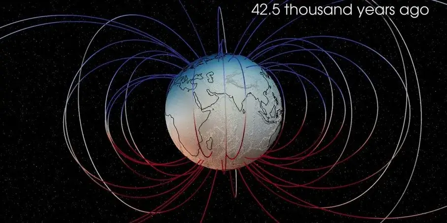
The original installation ran through a 32-speaker array in a public square in Copenhagen, each speaker representing field variation at a different point on the globe over the past 100,000 years. Online, the animation and stereo mix compress that into a single seventy-eight-second piece. The field lines deform. Blue patches, where flux enters the core, bloom across the southern hemisphere. Red patches scatter. Briefly, there are more than two poles. Nielsen mixed natural sounds, creaking wood, falling stones, into something that sounds neither electronic nor entirely organic.

The team’s peer-reviewed write-up of the project, Schanner, Nielsen, Bickerton, Panovska and Kervalishvili (2026), appeared in Frontiers in Earth Science (DOI: 10.3389/feart.2025.1727273) as “An audiovisual representation of a geomagnetic excursion for public engagement.” As of October 2025 the video had over one million views on YouTube, making it the ESA Earth Observation channel’s most popular video to date, plus more than 60,000 views on Instagram, according to the paper’s own engagement audit. It is the most accurate science communication tool the geomagnetism community has produced for a general audience: not a metaphor, not a simulation, but the field itself, translated into a medium that doesn’t require a PhD to feel.

In Mukhopadhyay’s office in Ann Arbor, the simulation cycles back to its starting frame. The dipole is intact. The aurora is a thin ribbon over the Arctic. The magnetopause holds at ten Earth radii. He clicks play. The poles begin to drift again. North slides south through Siberia, dives toward the equator over the Indian Ocean, fragments. Spain begins to glow.

A reversed-flux patch under Cape Town moves a few hundred meters westward.

It is the same field.

Frequently Asked Questions

When was the Laschamps excursion?

The Laschamps excursion occurred about 41,000 years ago. The full event lasted roughly 2,000 years, with the most dramatic dipole reduction and tilt concentrated in a window of about 300 years. The reversed-polarity phase itself lasted roughly 440 years, according to Sanja Panovska’s reconstruction presented at the EGU General Assembly in 2024.

Is the South Atlantic Anomaly a sign of a magnetic pole reversal?

No. ESA’s October 2025 Swarm results, led by Chris Finlay at DTU Space, found no sign of an impending reversal. The SAA is growing and splitting into two lobes, and it shares structural features with past excursions, but those features are necessary, not sufficient, conditions for a global polarity flip.

Did the Laschamps event cause Neanderthals to go extinct?

Almost certainly not as a primary cause. Cooper and Turney’s 2021 Science paper proposed the link, but formal rebuttals by Andrea Picin (Max Planck) and John Hawks (Wisconsin) showed that Neanderthal disappearance and most cited megafaunal extinctions were already underway thousands of years before the magnetic minimum and are better explained by other factors.

How fast is Earth’s magnetic field weakening?

The dipole is 9 percent weaker than it was in 1840, according to Finlay, Aubert and Gillet’s 2016 Nature Communications paper. That is real and measurable, but it sits within the range of natural variation observed across the Holocene. The South Atlantic Anomaly is weakening faster locally: a region southwest of Africa has lost intensity at an accelerated rate since 2020.

Could a Laschamps-scale event happen today?

It could, in principle. Geomagnetic excursions occur on roughly 10,000-to-100,000-year timescales, and the current dipole decline plus growing SAA share some early-stage features. There is no evidence one is imminent, but the geophysical preconditions are not unrelated to the present configuration of the field.

What would happen to satellites and the power grid if it did?

Satellites in low Earth orbit, including the more than 10,000 active Starlink spacecraft and most Earth-observation constellations, would face dramatically higher radiation doses for far longer fractions of each orbit. Power grids would be vulnerable to geomagnetically induced currents capable of damaging extra-high-voltage transformers; the 2008 U.S. National Academies report estimated $1–2 trillion in first-year impacts and 130 million people without power for a single major event of much smaller magnitude.

Where can I listen to the sound of the magnetic flip?

The GFZ Potsdam / DTU Space sonification of the Laschamps excursion is available at the GFZ project page. The peer-reviewed write-up by Schanner, Nielsen, Bickerton, Panovska and Kervalishvili appeared in Frontiers in Earth Science in 2026 (DOI: 10.3389/feart.2025.1727273).