Introduction

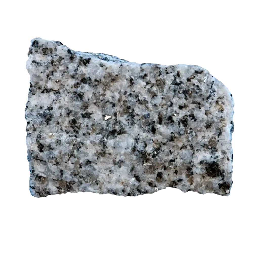
In the early 1990s, Phil Schmidt and George Williams ran a paleomagnetic experiment on red siltstone from the Elatina Formation in the Flinders Ranges of South Australia. The remanent magnetisation, locked in haematite grains roughly 635 million years ago, gave an inclination shallower than 10°. For a working paleomagnetist, the number is unambiguous. The rock was deposited within about 7° of the equator. The rock is a glaciomarine diamictite, striated clasts in a fine-grained matrix, dropstones puncturing laminae below, deposited where ice reached sea level.

That measurement, reproduced and corrected for sediment compaction in the years since, anchors one of the strangest claims in Earth science: that twice during the Cryogenian Period, for about 56 million years from 717 to 660 Ma (the Sturtian), then briefly around 635 Ma (the Marinoan, which the Elatina diamictite records in South Australia), ice sheets reached sea level at the equator. Grounded glaciers in the tropics, on a planet frozen pole-to-pole, and the rocks prove it. Two papers published in 2026, Minsky et al. in PNAS, Griffin et al. in EPSL, have now revised that consensus picture in different and complementary ways.

The rocks that prove the tropics froze

Four independent lines of evidence force the Snowball conclusion, and they have to be addressed together because each on its own can be argued away.

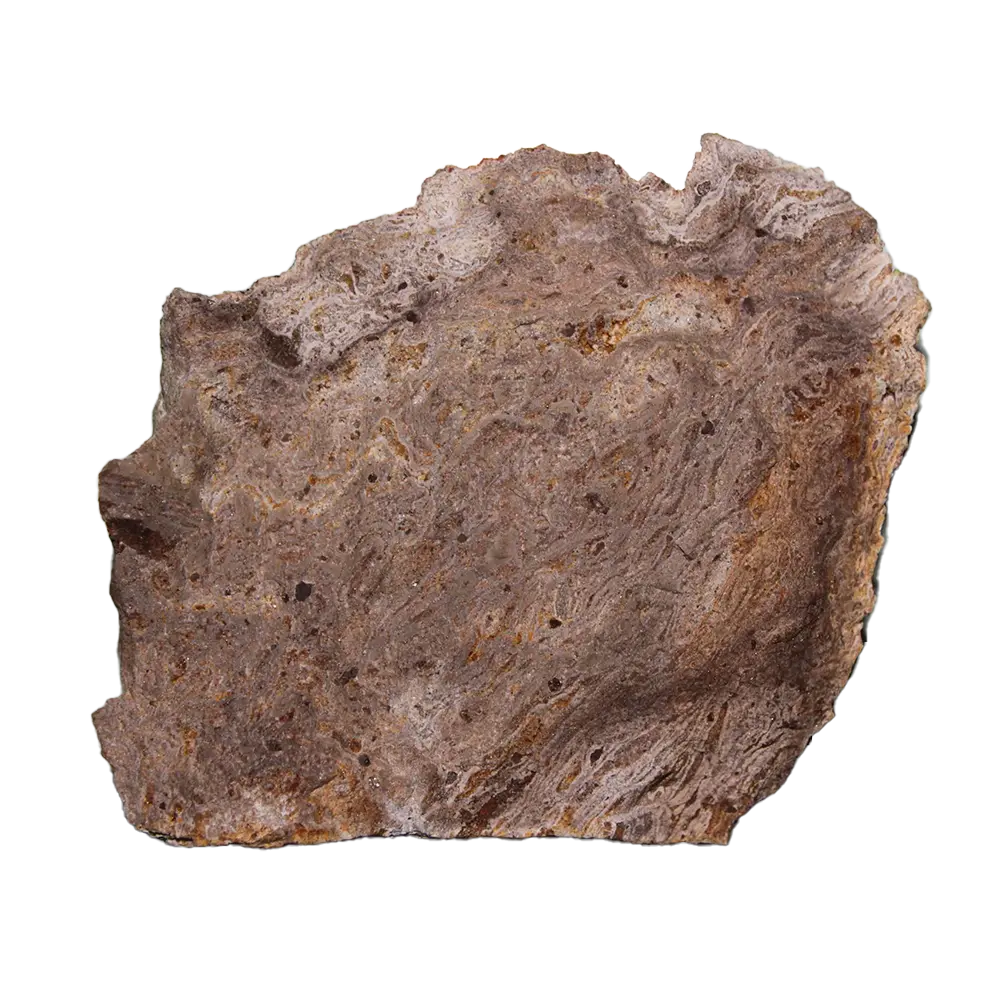
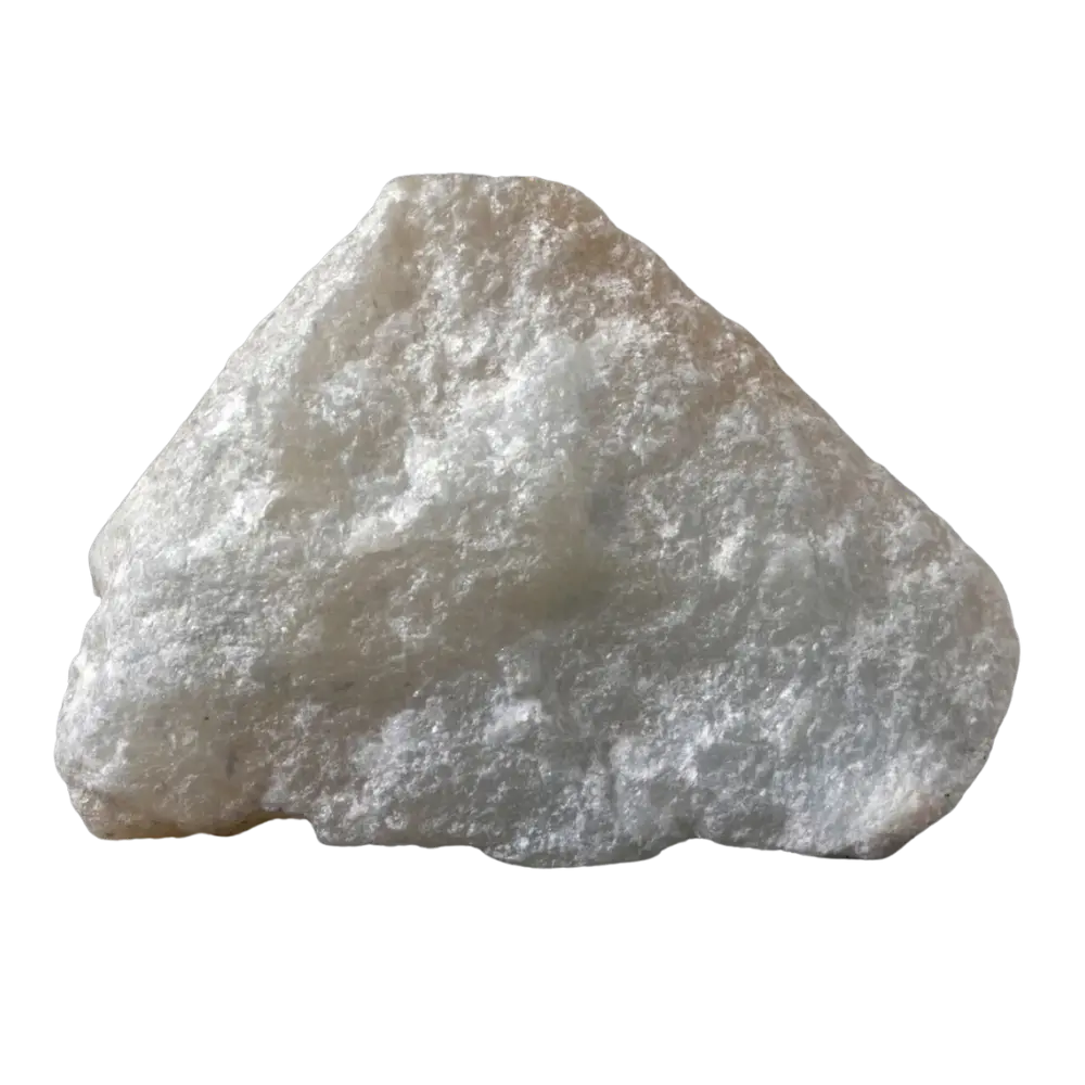
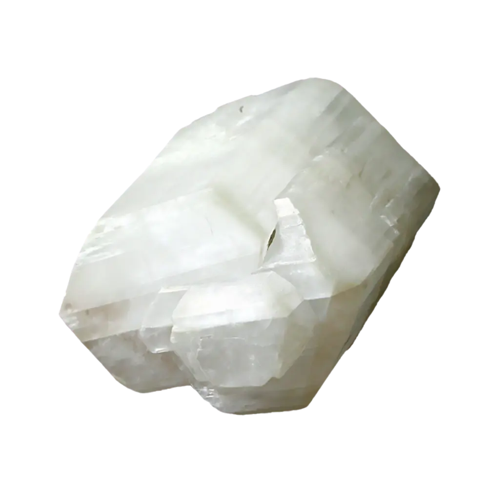
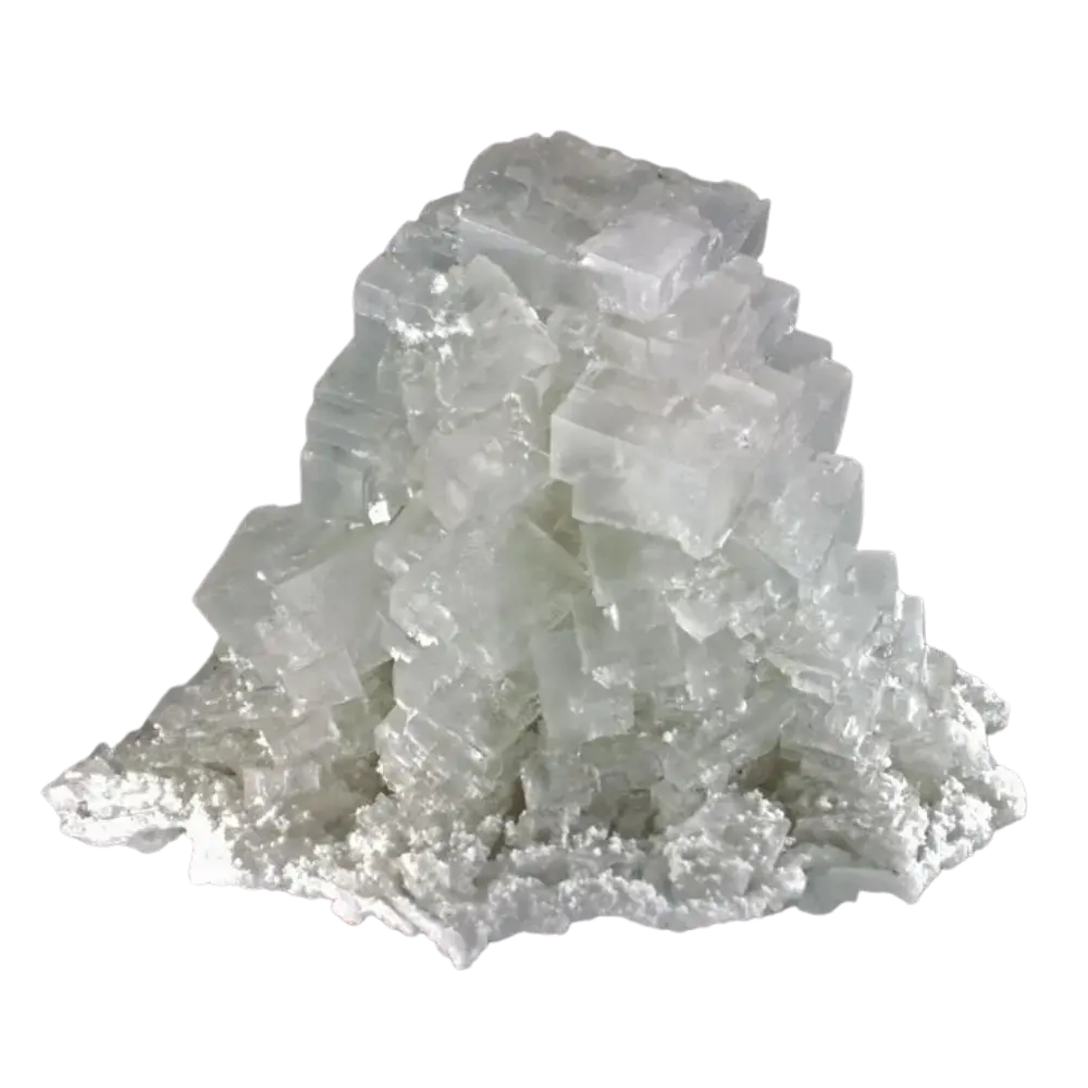
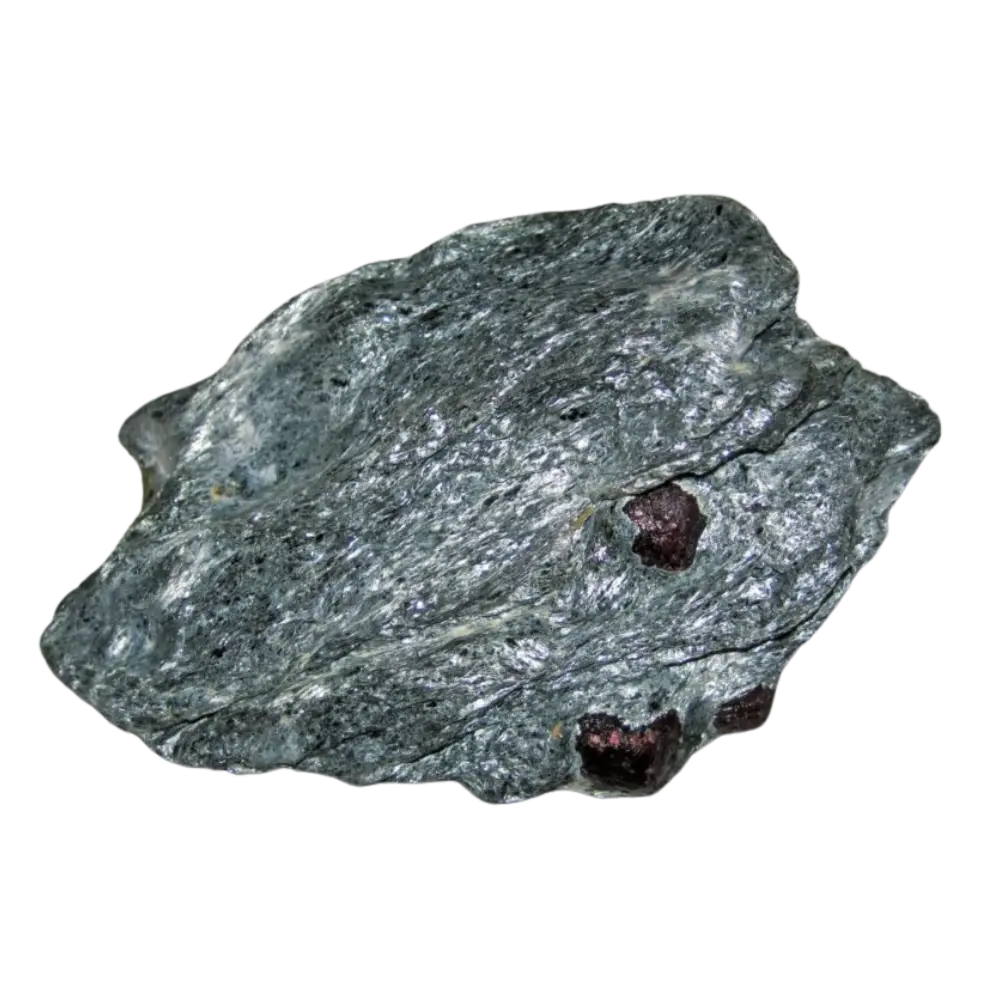
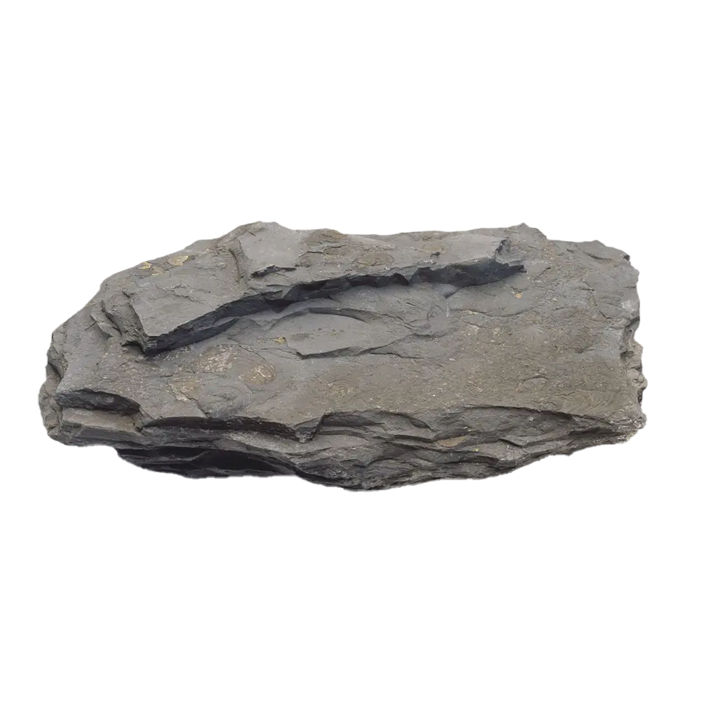
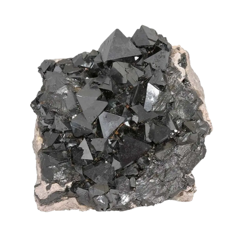
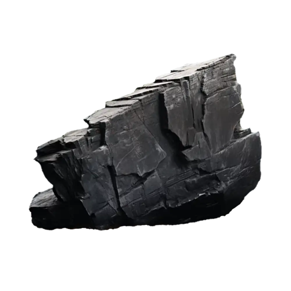
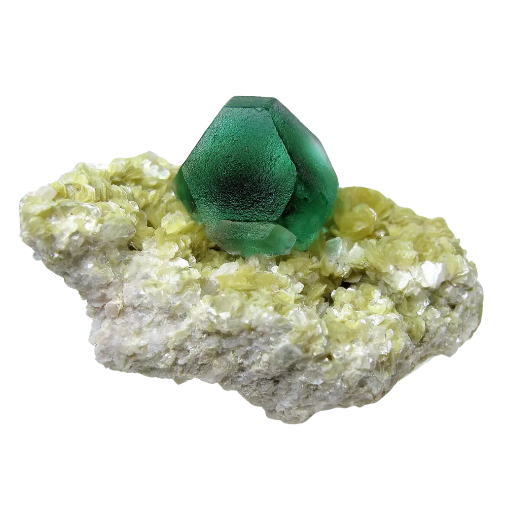
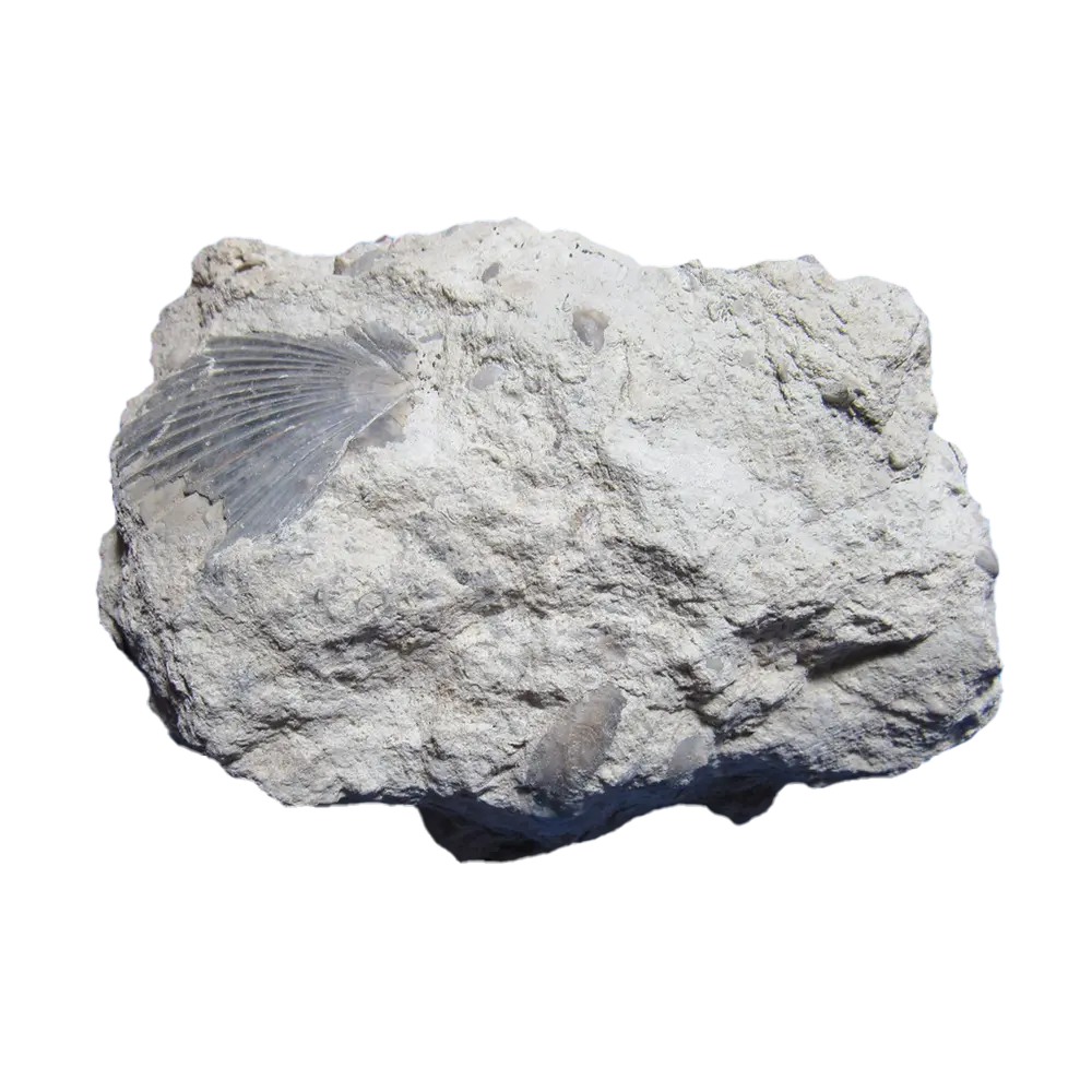
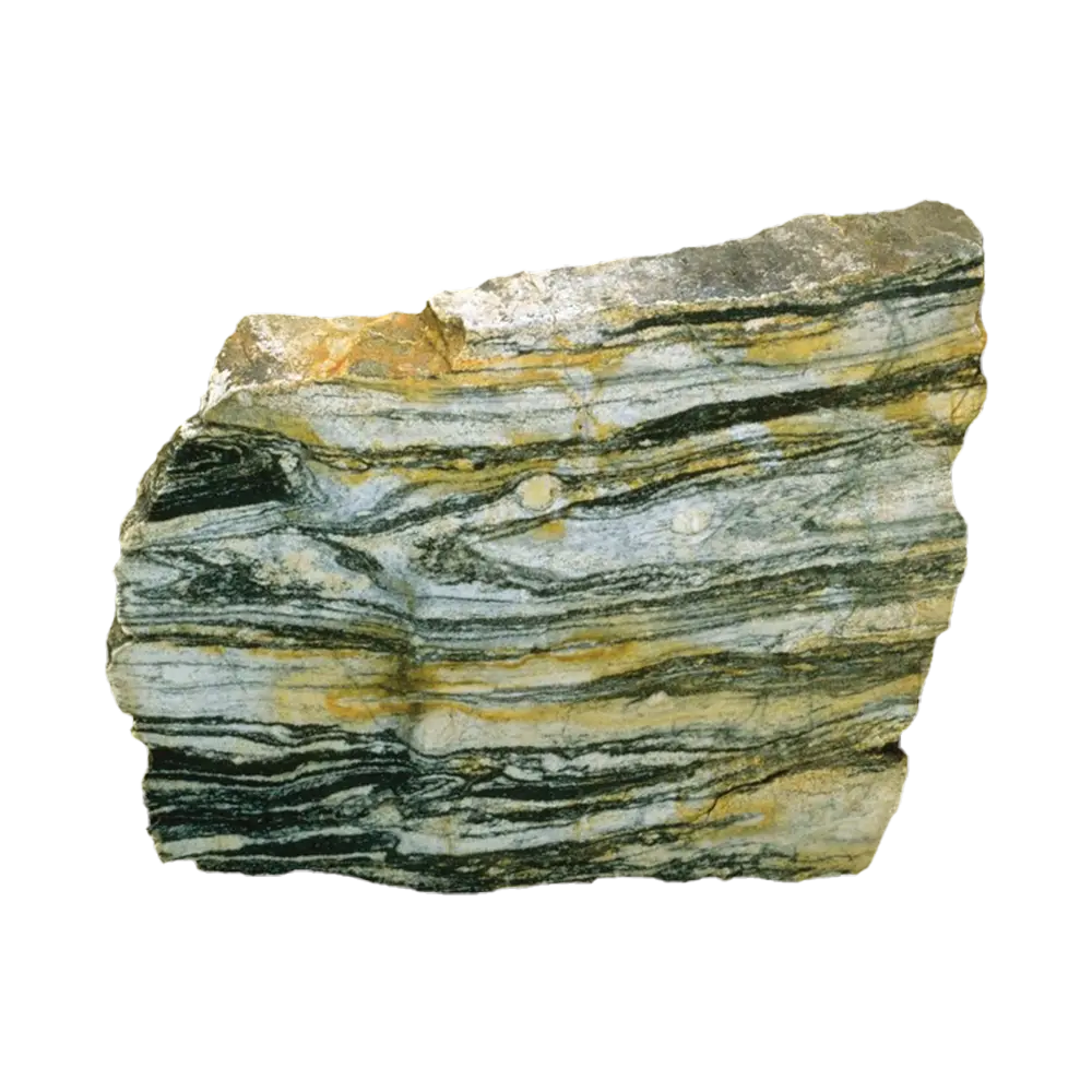
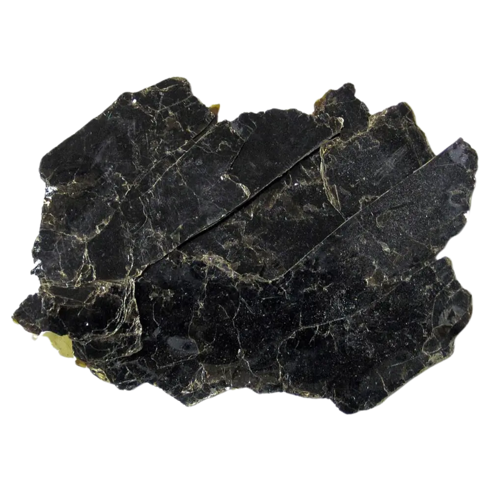
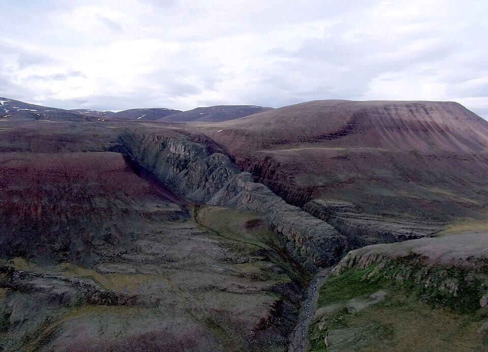
The first is the rock. Diamictites, poorly sorted, matrix-supported, pebble-to-boulder deposits with striated and faceted clasts, appear in Cryogenian sections on every continent that preserves them. The Elatina Formation in South Australia, the Ghaub and Chuos formations in Namibia, the Port Askaig in Scotland, the Nantuo in South China, the Rapitan Group in the Yukon. These are unambiguously glacial deposits. Dropstones puncture laminated mudstone underneath, recording icebergs calving into deep water.

The second is paleomagnetism. The Elatina data are not unique. Schmidt and Williams (1995), Sohl, Christie-Blick and Kent (1999), and more recent compilations all return shallow magnetic inclinations from glaciogenic Cryogenian rocks, implying paleolatitudes within roughly 10° of the equator. Hoffman, Kaufman, Halverson and Schrag (1998) put it bluntly in their Science paper: “Paleomagnetic evidence suggests that the ice line reached sea level close to the equator during at least two Neoproterozoic glacial episodes.” Macdonald et al. (2010) tightened this further by dating a rhyolite from the Mount Harper Volcanic Complex of Yukon at 717.4 ± 0.1 Ma, directly below the Rapitan glaciogenic strata, with paleomagnetic poles pinning Laurentia to an equatorial position at the time of deposition. Ice was grounded below sea level in the tropics.

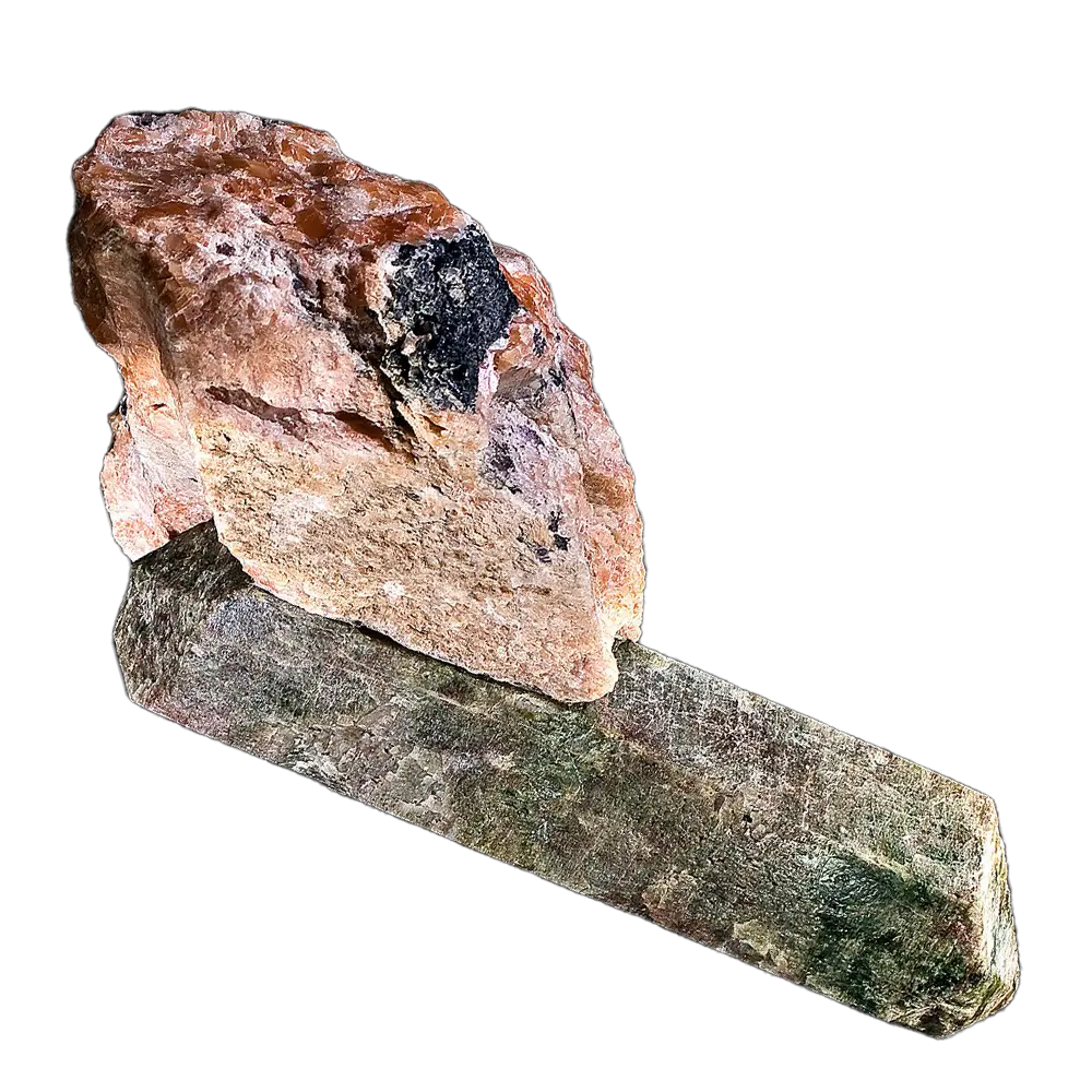
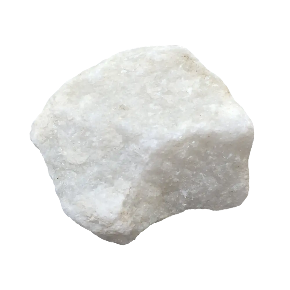
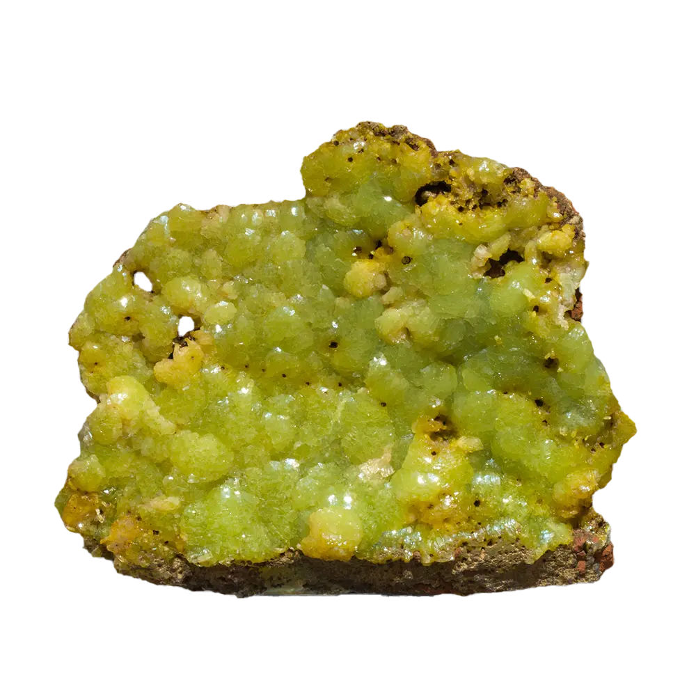
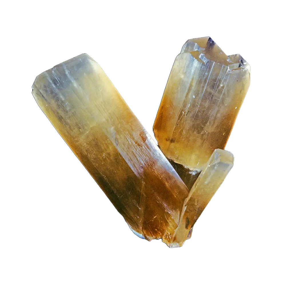
The third is the cap carbonate. Each Cryogenian glacial unit is overlain, sharply, almost violently, by a few tens of metres of dolostone or limestone with sedimentary textures that have no Phanerozoic analogue. Centimetre-wide tubes stand perpendicular to bedding. Wave ripples reach metre-scale wavelengths. Sheet cracks, opened by some still-unsettled mechanism, are filled with carbonate cement. Hoffman et al. (1998) read these as the precipitate of an ocean suddenly exposed to a hothouse atmosphere stuffed with volcanic CO₂.

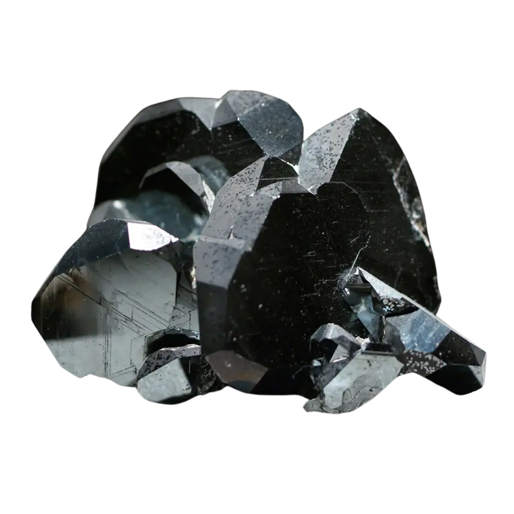
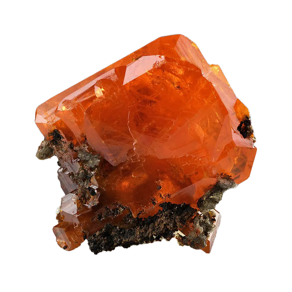
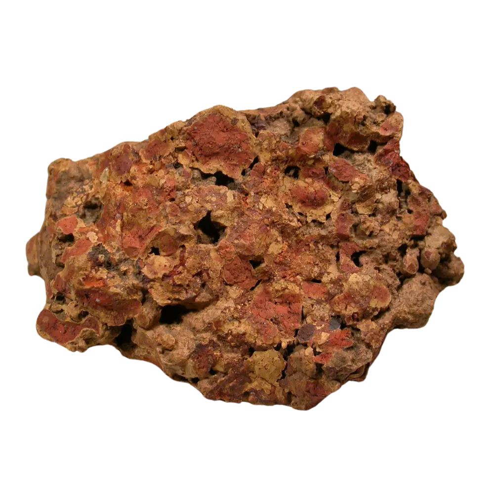
The fourth is the return of banded iron formation. BIFs vanish from the rock record around 1.85 Ga and re-appear, briefly, inside Sturtian successions like the Rapitan Group and the Holowilena Ironstone. A sea covered by thick ice cuts off oxygen exchange. Ferrous iron, sourced from hydrothermal vents, accumulates in the deep ocean until deglaciation oxidises it. Joseph Kirschvink flagged this exact pattern in the paragraph that named the hypothesis.

Kirschvink’s 1992 paragraph and Hoffman et al.’s 1998 reframing

The phrase “snowball Earth” appears in print for the first time on pages 51 and 52 of The Proterozoic Biosphere, a 1,348-page volume edited by Bill Schopf and Cees Klein in 1992. The contribution is seven paragraphs long, unrefereed, and signed by Joseph Kirschvink at Caltech. Kirschvink linked the low-latitude glacial deposits to a Budyko-style ice-albedo runaway, explained the reappearance of banded iron formations as a consequence of an ice-sealed anoxic ocean, and sketched an exit: volcanic CO₂, accumulating because silicate weathering had shut down, eventually breaking the albedo lock.

For six years the idea sat largely unread. Then in August 1998 Paul Hoffman, Alan Kaufman, Galen Halverson and Daniel Schrag published “A Neoproterozoic Snowball Earth” in Science. They had been working the Otavi Group of northern Namibia, measuring carbon isotope ratios through hundreds of metres of carbonate platform straddling the Ghaub glaciation. They found a positive δ¹³C plateau running between +5 ‰ and +9 ‰ in the pre-glacial Otavi carbonates, a sharp negative excursion to about −5 ‰ across the glacial–postglacial boundary, with some intervals plunging close to mantle-input values. The pre-glacial Trezona anomaly preserved in the Trezona Formation of South Australia recovers from roughly −9 ‰ to near 0 ‰ just below the Marinoan diamictite, the largest pre-glacial δ¹³C shift documented in Earth history.

The Hoffman team read this as the isotopic fingerprint of an ocean whose biological productivity collapsed for millions of years. To restart the carbon cycle and precipitate the cap carbonates, they argued, deglaciation had to raise atmospheric CO₂ to about 350 times the modern level. This number, about 350 PAL, is one estimate among several from a specific 1998 scenario, and the modelling community has spent the intervening 28 years arguing about it.

The Hoffman et al. paper turned Kirschvink’s seven paragraphs into a research programme. It also drew sustained opposition: sedimentologists found evidence of dynamic ice and open water; biogeochemists could not see how anything aerobic survived; and for years modellers could not get their GCMs to deglaciate at any plausible CO₂ level.

How it started: Rodinia, the Franklin LIP, and basalt weathering at the equator

To freeze a planet you need to overwhelm the silicate weathering thermostat. The Cryogenian world supplied that opportunity in abundance.

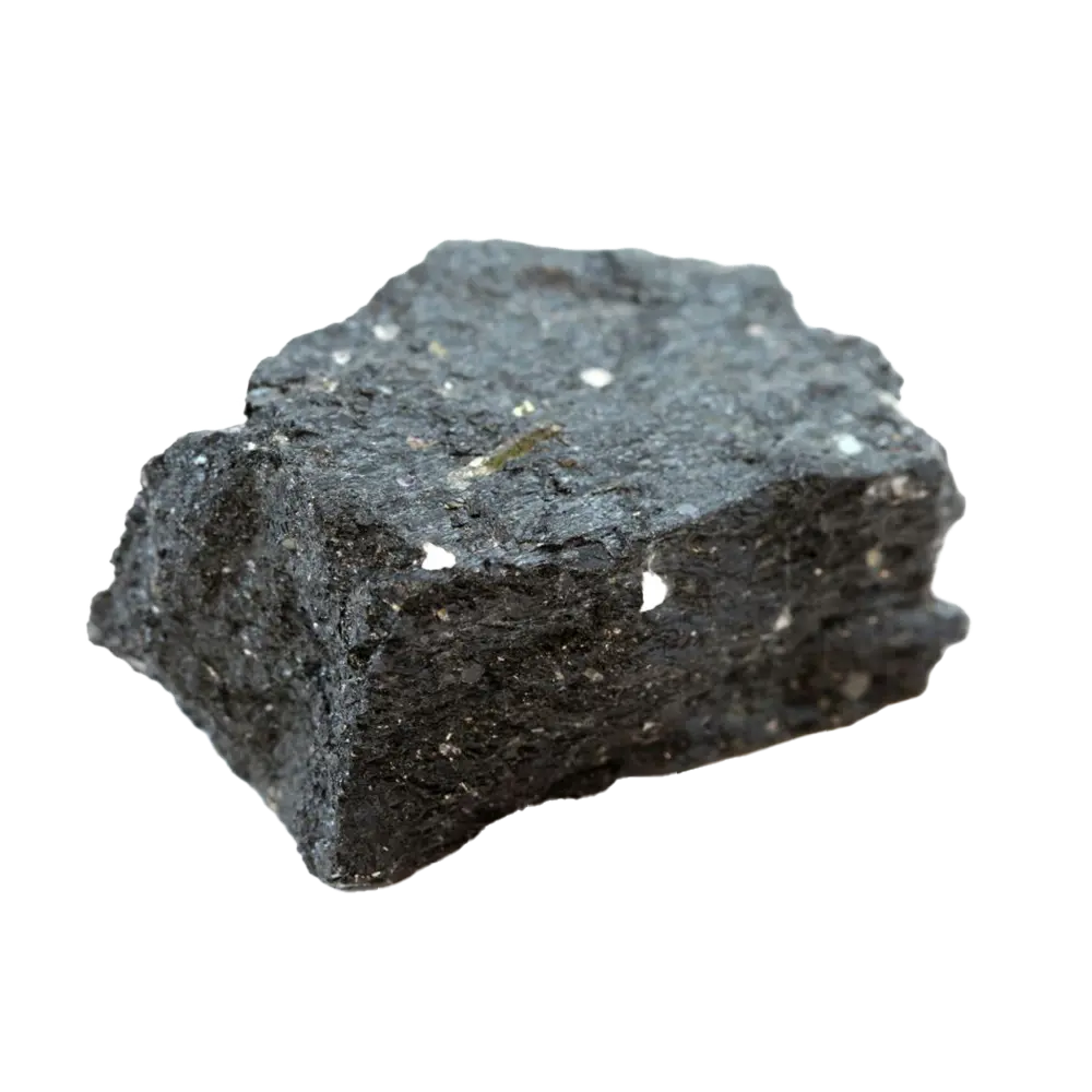
The supercontinent Rodinia had begun to fragment by about 800 Ma, and the new rifted margins were concentrated near the equator. Wet, warm continental crust at the equator is a chemical weathering engine. Then, between 719.86 ± 0.21 and 718.61 ± 0.30 Ma, the Franklin Large Igneous Province erupted across what is now Arctic Canada, Greenland, and the North Slope of Alaska. Dike swarms run for thousands of kilometres on Baffin Island and Victoria Island. Macdonald and Swanson-Hysell (2023) place the emplacement age within ~1–2 Myr of the Sturtian onset at 717.4 ± 0.1 Ma (Macdonald et al. 2010, with later refinements at 716.94 ± 0.24 Ma by Cox et al. 2018).

Fresh basalt at the equator does not last. It hydrolyses. Olivine and pyroxene break down to clay and dissolved cations, consuming atmospheric CO₂ at rates approximately 10 times higher than granite and gneiss (Dessert et al. 2001). Cox et al. (2016, EPSL) compiled Nd isotope data from mudstones in northern Rodinia that record exactly this drawdown signature in the run-up to the Sturtian. Their conclusion: “weathering of flood basalt provinces provided the final trigger for Snowball glaciation.”

Cooling produces ice, which raises albedo, which reflects more sunlight to space, which cools the planet further. Past a threshold latitude the loop runs away. Mikhail Budyko worked out the energy-balance version of this in 1969. Kirschvink, building on James Walker, Hal Marshall and James Kasting, recognised in 1992 that the runaway need not be theoretical.

What the planet looked like at −50 °C

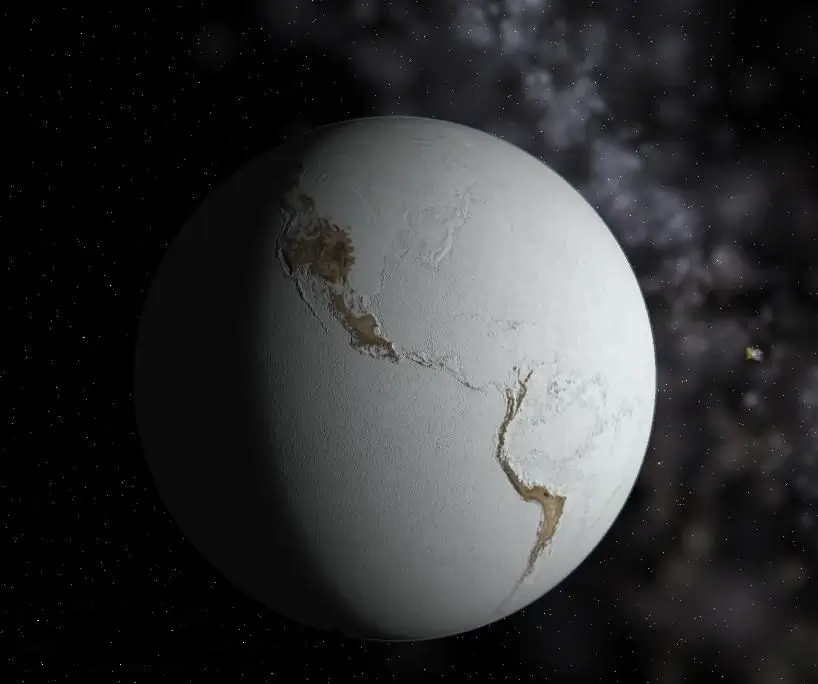
Hoffman et al. (2017, Science Advances) compiled the climate-dynamics literature into a quantitative picture of the Snowball mean state. Global mean surface temperature was roughly −50 °C. Their GCM runs were prescribed at a solar constant of 1,285 W m⁻², 94 percent of the present-day value, meaning the Sun was about 6 percent dimmer at the Sturtian onset than today. Sea-glacier ice, hundreds of metres thick, flowed equatorward from polar accumulation zones toward an equatorial ablation belt where it sublimated. The atmosphere held perhaps a thousandth of modern water vapour. Precipitation, where it fell, was as dry snow. The hydrological cycle did not stop, but it ran on a small fraction of modern throughput.

Continents were ice-covered to sea level, though the ice was thin in the dry tropics. High-latitude ice sheets overrode bedrock topography, while storm tracks compressed toward the equator. The Hadley circulation, modelled by Pierrehumbert in his 2005 JGR paper, took on a configuration with no Phanerozoic analogue.

The deep ocean, importantly, was not solid. Even with kilometre-thick sea ice, geothermal heat at the seafloor maintained liquid water beneath. Hydrothermal vents continued to operate. Bottom water sat near the freezing point of saline brine, around −2 °C. The base of the sea-ice never came near freezing the entire water column.

How life survived: refugia, cryoconite, and the modern deep biosphere as analogy

Life clearly survived. Eukaryotic microfossils, testate amoebae, vase-shaped microfossils, organic-walled acritarchs, are present in pre-Sturtian rocks and in post-Marinoan rocks. Animals appear after the Marinoan. Something carried the eukaryotic lineages through.

Candidates cluster around three kinds of refugia: marine, supraglacial, and chemoautotrophic-subglacial. The marine case turns on thin sea-ice or open-water polynyas near the equator where photosynthesis could continue. Lechte et al. (2019), studying iron-speciation in Sturtian iron formations from Australia, argued for at least some oxygenated near-shore water. Ye et al. (2023, Nature Communications), working on Marinoan-age fossils in the Nantuo Formation of South China, documented benthic photosynthetic macroalgae preserved in black shales interbedded with glacial diamictites, with iron-speciation and nitrogen-isotope data consistent with dysoxic-to-oxic mid-latitude coastal habitats during the waning Marinoan.

The supraglacial case rests on cryoconite pans. Hoffman’s 2016 Geobiology paper proposed these as dust-darkened meltwater holes on the equatorial sea-glacier surface, ringed by cyanobacterial mats, drained periodically into the subglacial ocean. Modern analogues exist on the McMurdo Ice Shelf, where Husain, Millar, Jungblut, Hawes, Evans and Summons (2025, Nature Communications 16, art. 5315) recovered steroid biomarkers and 18S rRNA gene signatures from sixteen photosynthetically active microbial mats in supraglacial meltwater ponds. The McMurdo ponds, they argue, serve as direct analogues for the refugia in which eukaryotic life could have ridden out the Cryogenian.

The subglacial and hydrothermal case is the most familiar in principle. Chemoautotrophic ecosystems around vents do not need surface sunlight, and the deep biosphere known from drilling Phanerozoic sediments is an existence proof that microbial life can sustain itself on rock–water reactions alone. It is not direct evidence for Cryogenian biota, but it removes one objection.

The Minsky et al. (2026) limit-cycle model has a separate, biological consequence here. If the Sturtian was not one continuous 56-Myr freeze but a sequence of shorter Snowball–hothouse swings, the oxygen problem softens considerably. Each hothouse interval lets photosynthesisers regroup and resupply atmospheric oxygen before the next freeze.

How a volcanic CO₂ rebuild flipped the planet back

The exit mechanism Kirschvink sketched in 1992 is now standard. Ice shuts down silicate weathering. Volcanic outgassing continues. CO₂ accumulates in the atmosphere over millions of years until the radiative forcing overcomes the high planetary albedo and the ice lines retreat.

The accumulating-CO₂ story leaves one number for the field to fight over: the deglaciation threshold pCO₂. Caldeira and Kasting (1992, Nature) ran a one-dimensional energy-balance model and found 0.12 bar was sufficient at present-day solar luminosity. Hoffman et al. (1998) used a different framing and quoted “about 350 times the modern level,” roughly 0.1 bar by partial pressure. Pierrehumbert (2004, Nature; 2005, JGR) ran the FOAM general circulation model and could not get his Snowball to deglaciate even at 0.2 bar, fingering cloud parameterisation as the likely culprit, a diagnosis later confirmed by Abbot et al. (2011, 2012). Hu et al. (2011) using CAM3 found different thresholds again. Wu, Liu, Hu and Yang (2021, JGR–Atmospheres) added explicit melt-pond physics and showed deglaciation can begin once annual-mean equatorial surface temperature reaches −7.7 °C, dropping the required pCO₂ to under 0.1 bar. Subsequent work adding orbital forcing has shown the deglaciation threshold pCO₂ varies by tens of thousands of ppmv depending on eccentricity and obliquity. Geochemical proxies independently constrain pCO₂ at the Marinoan termination to about 10² PAL, roughly 0.04 bar, tighter than any of the model estimates above (Hoffman et al. 2017).

Across this spread the qualitative story holds. The threshold sits between roughly 0.01 and 0.4 bar of CO₂, two to three orders of magnitude above modern. The exact value depends on cloud cover, surface dust, melt-pond physics, atmospheric pressure, and orbital configuration. The deglaciation is not gentle. Once the equatorial ice line begins to retreat, the same ice-albedo feedback that caused the freeze runs in reverse. Within a few thousand years, perhaps less, the planet enters the post-glacial hothouse with mean temperatures well above modern.

The hothouse is what precipitates the cap carbonates. Acid rain on freshly exposed silicate and carbonate continents delivers alkalinity to a CO₂-saturated ocean. Carbonate precipitates rapidly out of the surface ocean, blanketing the glacial diamictite globally. Karl-Heinz Hoffmann, Daniel Condon, Sam Bowring and Jim Crowley (2004, Geology) dated an ash bed within the Marinoan Ghaub Formation in Namibia at 635.5 ± 1.2 Ma using U-Pb on zircon, giving the deglaciation an effectively exact age. Independent U-Pb dates from Tasmania (636.41 ± 0.45 Ma, from the Cottons Breccia) and the basal Doushantuo cap in South China are within uncertainty of this figure, confirming globally synchronous Marinoan termination.

The 2026 Minsky et al. limit-cycle revision: solving the duration paradox

The duration of the Sturtian has been the field’s most stubborn puzzle. Rooney et al. (2014, 2015) used coupled Re-Os and U-Pb geochronology to bracket the glaciation between 717 and 660 Ma: about 56 to 58 million years. The Marinoan, by contrast, is brief. Tasistro-Hart, Macdonald, Crowley and Schmitz (2025, PNAS) used drone-mapped Marinoan stratigraphy in Namibia plus new radioisotopic dates to argue for a duration of about 4 Myr, with less than 10 m of vertical ice-grounding-line motion across glacial advance-retreat cycles. Other Marinoan estimates have ranged up to 15 Myr; the 4-Myr figure now has the best stratigraphic support.

Why a 14-fold difference? And why is 56 Myr a problem at all? Because every reasonable climate model says a hard Snowball should self-terminate in a few million years at most. The volcanic-CO₂-rebuild rate is constrained by mid-ocean-ridge and arc fluxes that are not arbitrary. At plausible degassing rates a hard Snowball should deglaciate in 5 to 15 million years. Fifty-six does not fit.

Charlotte Minsky, then a graduate student in Wordsworth’s group at Harvard SEAS, took on the puzzle directly. Their April 2026 PNAS paper, with co-authors David T. Johnston of Harvard’s Department of Earth and Planetary Sciences and Andrew H. Knoll of the same department and the Department of Organismic and Evolutionary Biology, used a coupled box model of Neoproterozoic climate and the global carbon cycle to ask whether the Sturtian could have been something other than one continuous freeze.

From the abstract: “Notably, new evidence indicates the Sturtian glaciation lasted for ∼56 Myr, far longer than can be accommodated by canonical ‘Snowball’ or ‘Slushball’ models.” And from the conclusion: “Thus, instead of a single, continuous Snowball, the climate repeatedly flipped between short, self-terminating Snowball glaciations and similarly short warm, largely ice-free interglacial climates.”

The mechanism is a limit cycle. Weathering of the freshly emplaced Franklin LIP basalts drove CO₂ down hard enough to push the climate into a Snowball. Inside the Snowball, weathering shut off and volcanic CO₂ rebuilt until the planet deglaciated into a hothouse. The hothouse exposed unweathered Franklin basalt again. Basalt weathering, accelerated by hothouse temperature and rainfall, drew CO₂ back down. The system re-entered a Snowball, and re-entered it again, for 56 million years: until the weatherable Franklin basalt inventory was exhausted.

Two consequences follow. First, the syn-glacial oxygen problem becomes tractable. Maintaining an oxygenated atmosphere across a continuous 56-Myr freeze — with a moribund biosphere reacting against volcanic reduced gases — has always been awkward; a limit cycle gives photosynthesisers repeated hothouse intervals to restock the atmosphere. Second, the limit cycle reproduces observed patterns of sedimentation: the intermittent open-water carbonates and ice-rafted debris documented within Sturtian successions, features hard to fit into a single motionless Snowball, now fit naturally.

The Minsky model keeps the Snowball; it just embeds it inside a cycle. Each Snowball phase, for its duration, is still the hard-frozen pole-to-equator state the geochemistry and paleomagnetism demand. The Sturtian becomes a sequence of them rather than one continuous freeze.

The 2026 Garvellach varves: a climate system still oscillating inside the deep freeze

Across the Atlantic from Harvard, on the windswept Garvellach Islands off the west coast of Argyll, the Port Askaig Formation exposes one of the cleanest Sturtian sections in the world. Elias Rugen has been mapping these rocks for five years. Chloe Griffin, lead author on the February 2026 EPSL paper, walked a single ~2,600-laminae unit and measured every couplet.

Each couplet is a varve: a coarse summer melt-season lamina topped by a fine winter drape, deposited annually into a deep, quiescent waterbody whose seasonal freeze-thaw cycle drove the sediment supply. From the abstract: “Our study indicates the laminites most likely represent annual varves, reflecting seasonal freeze-thaw cycles in a deep, quiescent waterbody. Spectral analysis of laminae thickness reveals decadal and centennial periodicities consistent with present-day Schwabe and Gleissberg solar cycles, alongside interannual periodicities, likely tied to ocean-atmospheric climate modes, resembling the modern El-Niño Southern Oscillation.”

The Schwabe cycle is the modern 11-year sunspot rhythm. The Gleissberg modulation is roughly 80 to 90 years long. Both fall out of the Port Askaig laminae-thickness spectrum, alongside shorter interannual peaks at two- to four-year periods. Griffin and colleagues compared the observations to fully coupled ocean–atmosphere model runs with Cryogenian paleogeography. Hard-Snowball runs reproduced the interannual peaks, atmospheric dynamics survive sea-ice cover, but only scenarios in which roughly 15 percent of the ocean surface remained ice-free reproduced the multidecadal signal. Minmin Fu, who led the coupled-model work at Southampton, put it this way in the press release: “You don’t need vast open oceans. Even limited areas of open water in the tropics can allow climate modes similar to those we see today to operate, producing the kinds of signals recorded in the rocks.”

Griffin and colleagues call this “resembling the modern El-Niño Southern Oscillation,” and the hedge matters. ENSO depends on a specific Pacific basin geometry that did not exist in the Cryogenian, so what they document is a periodicity in the ENSO band, not the modern Pacific phenomenon itself. The real claim is harder: some kind of ocean–atmosphere coupled mode was active during a Snowball episode, on a planet that until very recently was assumed too cold and too ice-locked for any such thing.

Gernon’s framing, in the press release, is measured: “It tells us the climate system has an innate tendency to oscillate, even under extreme conditions, if given the slightest opportunity.” Griffin and colleagues themselves treat the open-water interval as a short-lived disturbance, likely thousands of years long, against an otherwise frozen background, not a full hothouse phase. That reading sits comfortably alongside the Minsky cycle: even individual Snowball episodes can include intervals with enough tropical open water to sustain seasonal hydrology and the ocean–atmosphere coupling that produces interannual modes.

What it means today: tipping points, exoplanets, and the Slushball debate

The Snowball record sits at the intersection of several live questions. It documents an upper bound of plausible Earth variability, what the planet looks like when ice-albedo runaway wins, and ties continental flood basalts directly to the silicate-weathering thermostat. The habitability lesson is the one that travels furthest: Earth survived two pole-to-equator freezes and emerged with animals after the second. Icy exoplanets need not be sterile.

The Slushball/Snowball debate persists, and the 2026 papers do not close it. Slushball proponents argue that equatorial ocean stayed open even during peak glaciation, providing a continuous photic refuge. Hard-Snowball proponents argue that the geological evidence, particularly the magnitude of sea-level change implied by the Ghaub grounding-line wedge studied by Domack and Hoffman (2011), requires continuous global ice cover. The 2026 Minsky model is interesting here because it offers a third option: the planet may have been a hard Snowball part of the time and ice-free part of the time, with the rock record sampling both. The Griffin and Gernon varves do not need a permanently open tropical ocean; they need open ocean during the interval the Port Askaig laminae record, which the limit-cycle model accommodates.

None of this means another Snowball is around the corner. The Sun is roughly 6 percent more luminous now than at the Sturtian onset (Hoffman et al. 2017), and modern tropical continents are not concentrated equatorial flood basalts. What does carry over is narrower: the silicate-weathering thermostat has finite gain, and once ice-albedo feedback crosses its threshold, Earth’s climate can settle into states no Holocene analogue prepares us for.

Frequently asked questions

How long did Snowball Earth last?

There were two Cryogenian Snowball episodes. The Sturtian lasted from c. 717 to 660 Ma, about 56 to 58 million years (Macdonald et al. 2010; Rooney et al. 2015; reaffirmed by Minsky et al. 2026). The Marinoan ended at 635 Ma; Tasistro-Hart et al. (2025) constrained its duration to about 4 Myr, placing its onset around 639 Ma, narrower than the older c. 650 Ma upper bound. The Marinoan termination is dated at 635.5 ± 1.2 Ma by Hoffmann et al. (2004).

How cold was the Earth during Snowball intervals?

Climate-dynamics work compiled by Hoffman et al. (2017) puts global mean surface temperature at roughly −50 °C during peak Snowball conditions. The deep ocean stayed near the freezing point of saline brine (about −2 °C) because of geothermal heat from below.

Was the equator really frozen?

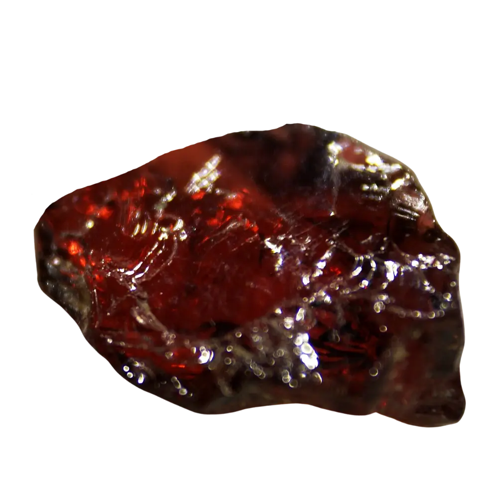
Yes, by the rock evidence. Paleomagnetic measurements on the Elatina Formation in South Australia (Schmidt and Williams 1995, with later compaction corrections) and a rhyolite dated by Macdonald et al. (2010) at 717.4 ± 0.1 Ma in the Yukon both show glaciogenic rocks deposited within about 10° of the equator, with Laurentia in equatorial position at the time of the Sturtian onset.

What triggered the Sturtian glaciation?

The leading hypothesis is chemical weathering of the Franklin Large Igneous Province, a flood basalt province emplaced across equatorial Laurentia between 719.86 ± 0.21 and 718.61 ± 0.30 Ma. Fresh basalt at the tropics consumes CO₂ at about ten times the rate of granite or gneiss (Dessert et al. 2001). Cox et al. (2016) compiled the Nd-isotope evidence; Macdonald and Swanson-Hysell (2023) refined the timing. The Sturtian onset followed within about 1 to 2 Myr.

How did the planet escape from the Snowball?

Volcanic outgassing kept supplying CO₂ to the atmosphere while ice shut down silicate weathering. After several million years CO₂ rose enough to overcome the ice-albedo feedback. Modelled deglaciation thresholds range from Caldeira and Kasting’s 0.12 bar (1992) to Pierrehumbert’s >0.2 bar (2004, 2005), with newer melt-pond and dust physics (Abbot and Pierrehumbert 2010; Wu et al. 2021) lowering the figure to under 0.1 bar. Hoffman et al. (1998) gave the original “about 350 times modern” estimate; Hoffman et al. (2017) derive a tighter geochemical bound of about 10² PAL (≈ 0.04 bar) at the Marinoan termination.

What does the 2026 Minsky et al. paper change?

Minsky, Wordsworth, Johnston and Knoll argue that the 56-Myr Sturtian was not one continuous freeze but a limit cycle of repeated short Snowball glaciations and short warm intervals, driven by Franklin LIP basalt-weathering swings. The model reconciles the duration with conventional climate dynamics, fits the observed sedimentary record, and softens the syn-glacial oxygen problem.

What did the Garvellach varves reveal?

Griffin, Gernon and colleagues (2026, EPSL) measured 2,640 annual laminae in the Port Askaig Formation and found Schwabe (~11-yr) and Gleissberg (~80–90-yr) solar periodicities alongside interannual ocean-atmospheric modes, indicating that coupled climate variability persisted during the Sturtian. Their coupled model runs match the multidecadal signal only when roughly 15 percent of the ocean surface remained ice-free.

How did life survive?

Through multiple refugia: thin sea-ice and open-water polynyas at low latitudes (Ye et al. 2023; Lechte et al. 2019); supraglacial cryoconite holes and meltwater ponds (Hoffman 2016; Evans et al. 2025); and chemoautotrophic ecosystems around hydrothermal vents in the still-liquid deep ocean. The Minsky limit-cycle model also implies repeated hothouse intervals that allowed surface biota to recover between freezes.