Introduction

The Great Dying took place 251.902 million years ago, and it is the closest thing the rock record offers to a planet-wide reset. Above the boundary, the bioclastic limestones full of brachiopod hash and crinoid debris give way to dolomitized microbial mounds and fine black shale. Conodont diversity drops sharply, with most Palaeozoic genera vanishing across a few centimetres of section.

The Great Dying, formally the end-Permian mass extinction, marking the Permian-Triassic boundary, eliminated more marine and terrestrial life than any other event in the Phanerozoic.

When Did the Great Dying Happen?

The Meishan section in Changxing County, Zhejiang Province, sits in an abandoned quarry on a low hill east of the village. It is the official Global Stratotype Section and Point for the base of the Triassic, ratified by the International Union of Geological Sciences in 2001. The boundary itself is defined biostratigraphically, placed at the first appearance of the conodont Hindeodus parvus in Bed 27c. Below that horizon, the rock holds a Palaeozoic fauna: fusulinid foraminifera, productid brachiopods, rugose corals, ammonoids. Above it, the survivors are a thinned-out menagerie of disaster taxa.

Six volcanic ash beds at Meishan have been dated by chemical-abrasion isotope-dilution thermal-ionization mass spectrometry on zircon. Shu-Zhong Shen and colleagues calibrated the extinction at Meishan to between 251.941 and 251.880 Ma. Seth Burgess, working with Sam Bowring and Shu-Zhong Shen at MIT, refined the boundary to 251.902 ± 0.024 Ma using high-precision U-Pb zircon dates from Meishan ash beds. A companion study cross-correlated the Meishan chronology to Siberian Traps zircons run through the same chemistry and the same mass spectrometer, removing the systematic biases that had hobbled earlier comparisons between Ar-Ar dates on the basalts and U-Pb dates on the Chinese boundary sections.

The Precision Closes the Causal Gap

A quoted uncertainty of ±24 kyr on a date 251.9 million years old is 0.01% relative error. It is the difference between knowing an extinction happened “around the Permian-Triassic boundary” and knowing whether it happened before or after a particular pulse of sill emplacement 4,500 kilometres away in Siberia. In deep time, causality is a geochronology problem. If the Siberian Traps post-date the extinction, they didn’t cause it. Pre-date it too far and the causal chain dissolves into noise. The Burgess–Bowring chronology placed the start of voluminous Siberian magmatism roughly 300,000 years before the marine extinction onset, with about two-thirds of the total magma volume emplaced before and during the extinction interval itself.

Pangaea Before the Catastrophe

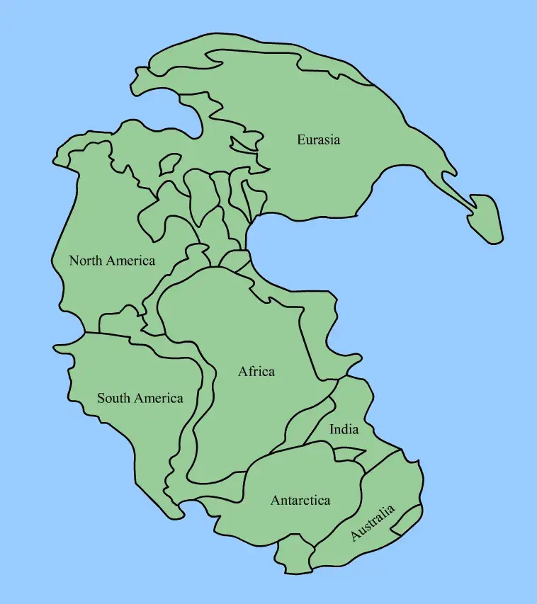
By the late Permian, every major continental block had collided into a single C-shaped supercontinent. Pangaea stretched from pole to pole, with the wedge of the Tethys Ocean opening eastward into Panthalassa, the global superocean covering roughly 70% of the planet’s surface. The interior was a megacontinental desert. Seasonal monsoons swept the coasts. Coal swamps of the Cathaysian flora persisted on the islands of South China and Indochina, and Glossopteris forests blanketed the southern Gondwanan latitudes.

Marine ecosystems in the latest Permian were biologically rich but structurally fragile. Reefs were built by calcareous sponges and tabulate-rugose coral assemblages, with Tubiphytes a prominent encrusting and binding component. The shelves of the Tethys, including the carbonate platforms now exposed in the Dolomites of northern Italy and in South China, supported diverse brachiopod, bryozoan, and crinoid communities. On land, the Karoo Basin of southern Africa preserves the most complete vertebrate record. The dicynodont therapsids Dicynodon and Diictodon grazed the floodplains; gorgonopsians like Inostrancevia and large therocephalians occupied the predator guild, while early cynodonts, the lineage that would eventually give rise to mammals, held smaller roles in the same assemblages.

Late Permian climate was already warming. Conodont oxygen isotope records from the Tethys margins show sea surface temperatures climbing from the latest Changhsingian into the earliest Triassic. Yadong Sun and colleagues, in a 2024 multiproxy and paleoclimate modelling study, used a doubling of atmospheric CO₂ from roughly 410 to 860 ppm across the latest Permian as the forcing scenario most consistent with proxy temperature records. The meridional overturning circulation weakened. The Hadley cell reorganized, with its descending branches shifting poleward. Climate forcing was already substantial in the latest Changhsingian, before Siberian magmatism reached its peak.

The Siberian Traps

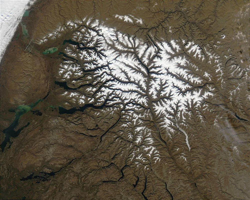
North of the Arctic Circle, beyond Norilsk, the Putorana Plateau rises in ridges of black-grey basalt cut by waterfalls that drop hundreds of metres down terraced cliffs. Each terrace is a separate lava flow. The Maymecha-Kotuy region to the east exposes stratigraphic sections more than three kilometres thick. Together these outcrops, along with the buried basalts of the West Siberian Basin imaged by hydrocarbon drilling, define the Siberian Traps Large Igneous Province. The province originally covered an estimated 5–7 million km², with current preserved exposures closer to 2–3 million km², and a preserved magmatic volume of around 3–4 million km³.

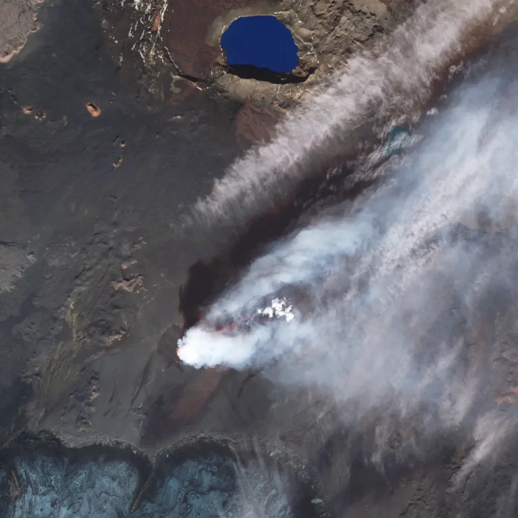
The eruption unfolded in phases. High-precision U-Pb dating by Burgess and Bowring divided the activity into phases. The earliest pyroclastic and volcaniclastic deposits, which built ash piles up to a kilometre thick in some areas, began around 252.24 Ma. Effusive flood basalts followed, with prodigious lava volumes emplaced in less than a million years. Lars Augland and colleagues, working with Norwegian and Russian field teams, used U-Pb zircon dates from intrusive complexes across Norilsk, Maymecha-Kotuy, and Taimyr to show that the main pulse of magmatism extended in both area and composition well beyond the classically mapped traps, with synchronous emplacement across distances of more than a thousand kilometres.

The mantle plume hypothesis remains the standard explanation. A deep thermal anomaly rose through the mantle, impinged on the base of the Siberian craton, and partially melted the lithospheric and asthenospheric mantle on a continental scale. The resulting magmas exploited pre-existing crustal weaknesses. Where they reached the surface, they erupted as basaltic curtains from fissures hundreds of kilometres long. Where they stalled in the upper crust, they spread laterally as sills.

Why the Siberian Traps Were So Lethal

By total magma volume, the Siberian Traps are not exceptional. The oceanic Ontong Java Plateau eclipses them; the Central Atlantic Magmatic Province of the end-Triassic was comparable in continental scale. What makes the Siberian event distinctive is where it erupted. The province sits atop the Tunguska Basin: Carboniferous-Permian coals, Cambrian and Devonian evaporites including bedded halite and anhydrite, and organic-rich shales, kilometres of carbon and sulphur waiting to be cooked.

Sills, Coal, and the Tunguska Basin Gas Bomb

Henrik Svensen and colleagues from the University of Oslo, working through the late 2000s, mapped more than 6,000 hydrothermal vent complexes piercing the Tunguska Basin sediments. The pipes are roughly cylindrical conduits, hundreds of metres in diameter and up to a kilometre tall, filled with brecciated country rock and lined with contact-metamorphic and hydrothermal mineral assemblages. Each pipe records the explosive venting of gas produced when an ascending sill cooked the sedimentary rocks it intruded. U-Pb dating of zircons in one such pipe placed the venting at 252.0 ± 0.4 Ma, coincident with the marine extinction at Meishan.

Heating Tunguska Basin coals to magmatic temperatures liberates methane and CO₂ on enormous scales. Heating the underlying halite-anhydrite evaporites does something more peculiar. Laboratory experiments by Svensen’s group on petroleum-bearing rock salt from Siberia showed that when natural evaporites are heated to about 275 °C, they release methyl chloride and methyl bromide. These are halocarbons with ozone-depleting potential comparable to or exceeding that of industrial CFCs.

Seth Burgess revisited the timing of the magmatism in 2017 and proposed a sharper hypothesis. The earliest phase of Siberian magmatism, dominated by surface lavas, predated the extinction by several hundred thousand years and did not, by itself, destabilize the biosphere. The crisis began when the magma plumbing changed. Around the time of the extinction onset, the dominant emplacement style switched abruptly from extrusive flood lavas to intrusive sills. Sills, unlike surface flows, intrude directly into sedimentary host rocks. Each sill becomes a giant thermal aureole. Burgess, James Muirhead, and Bowring argued that this initial pulse of laterally extensive sills cooked vast volumes of previously untapped, volatile-fertile sediment, releasing the carbon and sulphur volatiles that triggered the kill.

The geochemistry has since corroborated this picture. Ying Cui and collaborators used bulk carbon isotope records and an Earth system model to estimate the magnitude and rate of carbon emission across the boundary. Their best-fit scenario required a release on the order of tens of thousands of gigatons of carbon at peak rates of several Gt C yr⁻¹, with an isotopic signature consistent with a predominantly volcanic and contact-metamorphic source rather than a methane-clathrate trigger. Mercury anomalies in marine sediments tell the same tale. Jun Shen and colleagues measured mercury concentrations and isotopes across the Permian-Triassic boundary in ten marine sections spanning the Northern Hemisphere and Tethys. They found Hg peaks coincident with the extinction in shallow-water sections, while deep-water sections recorded Hg anomalies tens of thousands of years earlier, indicating that volcanism was already loading the atmosphere before biotic collapse became unambiguous in shelf assemblages.

Stephen Grasby and colleagues found a still-more disturbing line of evidence in Sverdrup Basin sediments of the Canadian High Arctic: layers of carbonaceous spherules indistinguishable under the microscope from modern coal fly ash, the residue of pulverized coal combusted at high temperatures. Their interpretation was that thermal eruptions through Tunguska coals lofted ash globally, dispersing toxic particulates over the oceans and contributing further metals to surface waters at exactly the time the marine biosphere was beginning to fail.

How a Mega El Niño Killed the Oceans

CO₂ forcing alone does not account for the scale of the kill. The mechanism that ties the carbon flux to 81% marine species loss is climatic and dynamical, working through ocean circulation, the Hadley cell, and tropical Pacific variability. A 2024 study in Science by Yadong Sun, Alexander Farnsworth, Michael Joachimski, Paul Wignall, Leopold Krystyn, David Bond, Domenico Ravidà, and Paul Valdes proposed what may be the most compelling reconstruction yet. Their integrated isotope and paleoclimate-modeling approach showed that as CO₂ doubled in the latest Permian, the equator-to-pole temperature gradient collapsed, the meridional overturning circulation weakened, the Hadley cell contracted, and the El Niño–Southern Oscillation grew pathological.

In their reconstruction, individual events lasted on the order of a decade, far beyond anything in the modern ENSO record, with tropical Pacific sea surface temperature anomalies large enough to redraw the rainfall map of Pangaea. Drought intervals stretched too long for tree species to survive between wet phases. In the oceans, the absence of meridional gradients and the slowing of overturning starved deep waters of oxygen while pushing surface temperatures past the thermal tolerances of plankton. The feedback compounded: dying forests stopped sequestering carbon, leaving more CO₂ in the atmosphere; more CO₂ produced still more intense ENSO swings; more intense ENSO swings killed more biomass.

The end-Permian extinction in the marine realm was not uniformly distributed across latitudes. Tropical taxa suffered, but extinction severity was higher at mid- and high latitudes for many marine groups. Justin Penn, Curtis Deutsch, Jonathan Payne, and Erik Sperling, in a 2018 paper in Science, modelled the Permian-Triassic ocean using a coupled climate–ecophysiology framework. They calculated a Metabolic Index for representative animal taxa: the ratio of oxygen supply to oxygen demand for a given organism at a given temperature. Their model reproduced the observed extinction geography because the high latitudes lost their cold, oxygen-rich refugia. Tropical species could shift poleward as the tropics warmed; high-latitude species had nowhere left to go.

Anoxia at Depth, Hypercapnia at the Surface

Pyrite framboid records, uranium isotopes, and the geochemistry of redox-sensitive trace metals all converge on a single picture for the latest Permian ocean. Bottom waters across vast shelf areas of the Tethys and Panthalassa became anoxic or even euxinic, containing free hydrogen sulphide. The chemocline shoaled. Photic-zone euxinia, recorded by biomarkers like isorenieratane derived from green sulfur bacteria, episodically reached into the surface ocean in some sections. The combination of warming, deoxygenation, and sulphide build-up was a physiological vise.

The Marine Kill Curve: Anoxia, Hypercapnia, Acidification

The headline extinction figure has shifted over the past two decades. Older syntheses, including the much-quoted 96% marine species loss, were based on rarefaction analyses with substantial sampling biases. More recent consensus estimates, including those drawn from the Paleobiology Database and from regional syntheses by Steven Stanley and Shu-Zhong Shen, place marine species loss at approximately 81%, with genus-level loss closer to 56%. The “Great Dying” framing remains accurate; the precise percentage shifts as fossil databases improve.

The kill curve is unevenly distributed across taxonomic groups. Heavily calcifying organisms with limited physiological buffering capacity suffered most. Rugose and tabulate corals were extinguished entirely. Fusulinid foraminifera and trilobites disappeared. Articulate brachiopods, which had dominated benthic shelf communities for 250 million years, lost most of their diversity. Mollusca came through with heavy losses but with enough survivors to seed the Mesozoic. Conodonts, ammonoids, and a handful of foraminiferal lineages provided the biostratigraphic backbone for correlating earliest Triassic sections.

Hana Jurikova and colleagues at GEOMAR in Kiel quantified ocean acidification across the boundary using boron isotopes in Late Permian brachiopod shells from the Southern Alps. The shells, deposited on the Tethys shelf of what is now northern Italy, recorded a substantial decline in seawater pH coincident with the onset of the mass extinction. Coupled with carbon isotope data and embedded in a geochemical model, the boron record resolved at least two distinct acidification pulses. The initial pulse, tied to rapid carbon release from the Siberian sill intrusions, was sharp enough to drive the carbonate saturation state of surface waters sharply downward within a few thousand years.

For shelled animals, acidification meant elevated metabolic costs of biomineralization. For animals already coping with elevated temperatures and reduced oxygen, the additional load of hypercapnia (high blood CO₂) pushed many physiologies past their tolerances. Jonathan Payne and Lee Kump argued years earlier that the selectivity pattern of the end-Permian extinction in the marine realm closely tracked the physiological capacity of taxa to buffer internal acid-base chemistry. Foster and colleagues, in a 2022 paleobiology study, used machine learning on a large marine fossil dataset and found that ecological traits associated with metabolic and respiratory limitation predicted extinction risk better than taxonomic affiliation.

Benjamin Black, working with Linda Elkins-Tanton, Erik Hauri, and Steven Brown, examined sulphur isotope ratios in melt inclusions trapped in Siberian Traps minerals to estimate sulphur emissions from the volcanic system. They concluded that the magmas carried substantially more sulphur than mantle-derived basalts typically do, with isotopic signatures pointing to evaporite-derived sulphate as an extra source. When that sulphur was injected into the stratosphere, it formed sulphate aerosols that scattered sunlight and produced episodes of regional cooling. When it returned to the surface, it produced acid precipitation across the Northern Hemisphere. Black, Jean-François Lamarque, and colleagues modeled the atmospheric chemistry of pulsed Siberian Traps degassing and found that the simulated rainfall reached pH values comparable to undiluted lemon juice over the eruption region, with episodes of global ozone depletion driven by halogen-bearing volatiles.

The Terrestrial Collapse and the Lystrosaurus Earth

On land, the end-Permian extinction is read most clearly in the Karoo Basin of South Africa. The Karoo’s Beaufort Group preserves a near-continuous floodplain succession from the late Permian through the early Triassic. Vertebrate biostratigraphy divides this interval into assemblage zones named after their characteristic genera. The Daptocephalus Assemblage Zone, late Changhsingian in age, is dominated by large dicynodonts and a diverse guild of gorgonopsian predators. Above it, in the Lystrosaurus Assemblage Zone, the fauna has been reduced to a handful of taxa, with the pig-sized dicynodont Lystrosaurus accounting for as much as 95% of identifiable specimens in some bone beds.

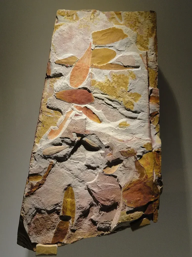
Lystrosaurus is the disaster taxon par excellence. Burrowing, opportunistic, and physiologically tolerant of low oxygen and elevated CO₂, it spread across Pangaea in the earliest Triassic with extraordinary efficiency. Its fossils have been recovered from Antarctica, India, China, European Russia, and South Africa, marking a near-cosmopolitan distribution. The Antarctic specimens, recovered by Edwin Colbert’s team at Coalsack Bluff in 1969, became one of the most-cited paleontological confirmations of continental drift. The post-extinction floodplains of the Karoo are essentially a Lystrosaurus monoculture, populated by a few small temnospondyl amphibians and the early therocephalian and cynodont survivors that would eventually radiate into the Mesozoic synapsid lineages.

The plant record is more nuanced. Cindy Looy and colleagues documented the collapse of the Glossopteris-dominated forests of southern Pangaea and the Cathaysian rainforests of the equatorial belt. Palynological assemblages across the boundary show abrupt replacement of pollen-producing gymnosperms by lycophyte and fern spores, the classic “fern spike” that marks post-disturbance landscapes. Soil erosion increased markedly, recorded as kaolinite-rich palaeosols and unusual coarse-grained alluvial deposits across multiple basins. Coal deposition essentially ceased globally for several million years, the “Early Triassic coal gap.”

Did the Land and Sea Extinctions Happen at the Same Time?

One of the more important shifts in our understanding of the Great Dying came from a 2024 paper by Qiong Wu and colleagues in Science Advances. Working on terrestrial Permian-Triassic sections in South China and North China, they applied high-precision U-Pb zircon dating to ash beds tied directly to fossil-bearing horizons. Their result: the main end-Permian terrestrial extinction in the paleotropics postdated the onset of the marine extinction by tens of thousands of years. The classic assumption of global synchronous collapse, with land and sea expiring together, does not hold in the equatorial belt.

That diachrony fits the mega El Niño model. Sun and colleagues argued that the mega El Niño signature, with its tropical heat plumes and continental aridification, killed land plants and animals progressively as drought intervals lengthened past survival thresholds. Marine ecosystems were initially buffered by ocean thermal inertia and by deep cold reservoirs, succumbing only as warming, deoxygenation, and acidification compounded over the following tens of thousands of years. The Karoo’s vertebrate record, studied by Roger Smith, Jennifer Botha-Brink, and Pia Viglietti, shows a stepwise collapse rather than a single horizon, with the dominant gorgonopsian predators disappearing before the dicynodont prey base.

What Caused the End-Permian Extinction?

The evidence converges from six independent directions. U-Pb dates on Siberian sills and on Meishan ash beds, run in the same laboratory, place the initial sill intrusion roughly 300 kyr before the marine extinction onset, with the dominant magma emplacement style switching from extrusive lavas to intrusive sills at the boundary itself. Boron isotopes from Tethys-margin brachiopods record acidification pulses synchronous with that emplacement change. Mercury anomalies in marine sediments worldwide spike at the same horizon. Carbon isotope excursions, modelled by Cui and colleagues, require a roughly 36,000 Gt carbon release with a volcanic isotopic signature at rates near 5 Gt C yr⁻¹. Sulphur isotopes from Siberian melt inclusions show heavy loading of evaporite-derived sulphate. Coal fly ash residues in Canadian Arctic sediments record combustion of Tunguska coals on a continental scale.

Each line of evidence builds on the others. A mantle plume rises under the Siberian craton. Sills intrude a sediment package loaded with coal, evaporites, and organic shale. The atmosphere takes on CO₂, methane, methyl halides, and sulphate aerosols. Warming, acidification, and runaway ENSO dynamics follow. Marine and terrestrial communities collapse.

For comparison, modern anthropogenic carbon emissions are running at roughly 10 Gt C yr⁻¹, twice the peak rate Cui and colleagues estimated for the end-Permian. The total cumulative budget of the Siberian Traps degassing exceeds anything humans could plausibly emit by burning all known fossil fuel reserves. Human emissions will not reproduce the Siberian Traps budget. What the rock record warns about is rate, the feedbacks that engage when a planet’s carbon system is perturbed faster than its buffers can respond.

Recovery, and Why It Took 10 Million Years

The earliest Triassic ocean was a strange place. Carbonate platforms in South China and Iran are dominated by microbialites: laminated and clotted carbonate fabrics produced by cyanobacterial mats. These are typical of Precambrian seas, before grazing animals kept microbial communities suppressed on shallow shelves. In the immediate aftermath of the extinction, with grazers and reef-builders gone, microbialites returned as the dominant marine carbonate factory. Bivalve assemblages were monotonous, dominated by a few opportunist genera such as Claraia and Eumorphotis. Ammonoid diversity, having collapsed across the boundary, rebounded numerically within a million years but remained ecologically narrow for far longer.

Surface ocean temperatures, reconstructed from conodont apatite oxygen isotopes by Joachimski and others, remained extraordinarily high through the early Triassic. Tropical sea surface temperatures approached 40 °C in the Smithian (Sun et al. 2012 Science.), conditions that excluded most large fish and tetrapods from the equatorial oceans entirely. The Early Triassic “tropical dead zone” lasted several million years before temperatures eased enough to permit diverse marine communities to reoccupy low latitudes.

Mercury records compiled by Shen and colleagues across multiple sections show that Siberian Traps magmatism continued in pulses well into the Early Triassic, with at least two distinct post-extinction events. Each pulse seems to have prolonged or reset the recovery. Anoxia returned. Carbon isotope curves oscillated wildly through the early Triassic, indicating sustained perturbation of the global carbon cycle. The Burgess–Bowring chronology shows that surface volcanism continued for at least another 500,000 years after the extinction ended, and the volume of post-extinction magma rivalled what came before.

Complex reef ecosystems did not reappear until the Middle Triassic, roughly 7 to 10 million years after the Permian-Triassic boundary, with the rise of scleractinian corals replacing the extinct rugose-tabulate guild. The recovery interval represents the longest such hiatus in the Phanerozoic, longer than the recovery from any other mass extinction. The recovery from the end-Cretaceous Chicxulub event, by comparison, was largely complete within several million years for most marine and terrestrial groups

What the Permian-Triassic Boundary Tells Us About Modern Climate

The Permian-Triassic boundary now appears in IPCC chapters on ocean ecosystem response. Climate scientists read it as the rock record’s cleanest example of a planet driven into collapse by carbon-cycle perturbation, high CO₂, low oxygen, low pH, and warm.

Penn, Deutsch, Payne, and Sperling framed their temperature-dependent hypoxia work against modern ocean deoxygenation trends. Researchers compare Jurikova’s boron-isotope record from Tethys brachiopods directly with modern boron-isotope pH reconstructions from coral skeletons. Cui’s carbon emission rates appear in policy literature next to contemporary fossil fuel figures.

The numbers don’t map cleanly onto today. The Siberian Traps released their carbon over hundreds of thousands of years, with a cumulative budget no human fossil fuel scenario could approach. Pangaea is gone. The polar ice masses that buffer modern warming did not exist. No mantle plume has surfaced beneath a coal-and-evaporite basin in our hemisphere.

What does map is rate. Anthropogenic emissions are running at roughly twice the peak rate Cui estimated for the Siberian event. The Permian-Triassic record shows what happens when ocean chemistry is perturbed faster than its buffers respond.

What We Still Don’t Know About the Permian-Triassic Extinction

Some pieces of the end-Permian extinction story remain unresolved. The role of methane clathrate destabilization has been argued back and forth for two decades; the Cui isotope analysis disfavours a major clathrate input, though it does not rule out a contribution. The relative importance of marine anoxia, hydrogen sulphide poisoning, and warming as marine kill mechanisms continues to be debated taxon-by-taxon. The terrestrial extinction in southern high latitudes, in places like the Sydney Basin of Australia and the Bowen Basin, appears to have begun even before the Karoo and Chinese events, suggesting that the global terrestrial collapse was diachronous in both directions.

Field campaigns continue. New Permian-Triassic boundary sections are being measured in the Canadian Arctic, in Iran, in Turkey, in Oman, and in the deep-ocean Panthalassic sections preserved as accreted blocks in Japan. Each adds a regional dimension to the global story. The thin clay layer at Meishan remains the type specimen, the rosetta stone against which everything else is calibrated. But it is no longer the only rock that matters.

The boundary at Meishan is a thin pale band of altered volcanic ash, the kind of thing you would walk past on a hillside without noticing. It records the conversion of a Palaeozoic biosphere of trilobites, brachiopod-dominated shelves, and Glossopteris forests into a depopulated Mesozoic stage on which Lystrosaurus rooted across floodplains and microbialites grew over the wreckage of the reefs. The killing phase lasted on the order of 60,000 years. The recovery took ten million.

Frequently Asked Questions

When did the Great Dying happen? 251.902 ± 0.024 million years ago, at the boundary between the Permian and Triassic periods.

What caused the end-Permian mass extinction? The Siberian Traps Large Igneous Province, particularly the intrusion of magma sills into coal, evaporites, and organic-rich shales of the Tunguska Basin, which released roughly 36,000 gigatons of carbon along with sulphur, halocarbons, and toxic metals.

How many species went extinct? Approximately 81% of marine species and 56% of marine genera. Terrestrial losses are harder to quantify but were comparably severe.

How long did the extinction last? The killing phase took roughly 60,000 years. The magmatic trigger spanned around 300,000 years before the marine extinction began. Full ecosystem recovery required 7 to 10 million years.

References

1. Burgess, S.D. & Bowring, S.A. (2015). High-precision geochronology confirms voluminous magmatism before, during, and after Earth’s most severe extinction. Science Advances, 1(7): e1500470. https://doi.org/10.1126/sciadv.1500470
2. Burgess, S.D., Muirhead, J.D. & Bowring, S.A. (2017). Initial pulse of Siberian Traps sills as the trigger of the end-Permian mass extinction. Nature Communications, 8: 164. https://doi.org/10.1038/s41467-017-00083-9
3. Sun, Y., Farnsworth, A., Joachimski, M.M., Wignall, P.B., Krystyn, L., Bond, D.P.G., Ravidà, D.C.G. & Valdes, P.J. (2024). Mega El Niño instigated the end-Permian mass extinction. Science, 385(6714): 1189–1195. https://doi.org/10.1126/science.ado2030
4. Wu, Q., Zhang, H., Ramezani, J., Zhang, F.-F., Erwin, D.H., Feng, Z., Shao, L.-Y., Cai, Y.-F., Zhang, S.-H., Xu, Y.-G. & Shen, S.-Z. (2024). The terrestrial end-Permian mass extinction in the paleotropics postdates the marine extinction. Science Advances, 10(5): eadi7284. https://doi.org/10.1126/sciadv.adi7284
5. Shen, S.-Z., Crowley, J.L., Wang, Y., Bowring, S.A., Erwin, D.H., Sadler, P.M., Cao, C.-Q., Rothman, D.H., Henderson, C.M., Ramezani, J., Zhang, H., Shen, Y., Wang, X.-D., Wang, W., Mu, L., Li, W.-Z., Tang, Y.-G., Liu, X.-L., Liu, L.-J., Zeng, Y., Jiang, Y.-F. & Jin, Y.-G. (2011). Calibrating the end-Permian mass extinction. Science, 334(6061): 1367–1372. https://doi.org/10.1126/science.1213454
6. Bowring, S.A., Erwin, D.H., Jin, Y.G., Martin, M.W., Davidek, K. & Wang, W. (1998). U/Pb zircon geochronology and tempo of the end-Permian mass extinction. Science, 280(5366): 1039–1045. https://doi.org/10.1126/science.280.5366.1039
7. Cui, Y., Li, M., van Soelen, E.E., Peterse, F. & Kürschner, W.M. (2021). Massive and rapid predominantly volcanic CO₂ emission during the end-Permian mass extinction. Proceedings of the National Academy of Sciences, 118(37): e2014701118. https://doi.org/10.1073/pnas.2014701118
8. Penn, J.L., Deutsch, C., Payne, J.L. & Sperling, E.A. (2018). Temperature-dependent hypoxia explains biogeography and severity of end-Permian marine mass extinction. Science, 362(6419): eaat1327. https://doi.org/10.1126/science.aat1327
9. Black, B.A., Lamarque, J.-F., Shields, C.A., Elkins-Tanton, L.T. & Kiehl, J.T. (2014). Acid rain and ozone depletion from pulsed Siberian Traps magmatism. Geology, 42(1): 67–70. https://doi.org/10.1130/G34875.1
10. Svensen, H., Planke, S., Polozov, A.G., Schmidbauer, N., Corfu, F., Podladchikov, Y.Y. & Jamtveit, B. (2009). Siberian gas venting and the end-Permian environmental crisis. Earth and Planetary Science Letters, 277(3–4): 490–500. https://doi.org/10.1016/j.epsl.2008.11.015
11. Grasby, S.E., Sanei, H. & Beauchamp, B. (2011). Catastrophic dispersion of coal fly ash into oceans during the latest Permian extinction. Nature Geoscience, 4: 104–107. https://doi.org/10.1038/ngeo1069
12. Shen, J., Chen, J., Algeo, T.J., Yuan, S., Feng, Q., Yu, J., Zhou, L., O’Connell, B. & Planavsky, N.J. (2019). Evidence for a prolonged Permian-Triassic extinction interval from global marine mercury records. Nature Communications, 10: 1563. https://doi.org/10.1038/s41467-019-09620-0
13. Jurikova, H., Gutjahr, M., Wallmann, K., Flögel, S., Liebetrau, V., Posenato, R., Angiolini, L., Garbelli, C., Brand, U., Wiedenbeck, M. & Eisenhauer, A. (2020). Permian–Triassic mass extinction pulses driven by major marine carbon cycle perturbations. Nature Geoscience, 13: 745–750. https://doi.org/10.1038/s41561-020-00646-4
14. Black, B.A., Hauri, E.H., Elkins-Tanton, L.T. & Brown, S.M. (2014). Sulfur isotopic evidence for sources of volatiles in Siberian Traps magmas. Earth and Planetary Science Letters, 394: 58–69. https://doi.org/10.1016/j.epsl.2014.02.057
15. Erwin, D.H. (2006). Extinction: How Life on Earth Nearly Ended 250 Million Years Ago. Princeton University Press, Princeton, NJ.
16. Foster, W.J., Ayzel, G., Münchmeyer, J., Rettelbach, T., Kitzmann, N.H., Isson, T.T., Mutti, M. & Aberhan, M. (2022). Machine learning identifies ecological selectivity patterns across the end-Permian mass extinction. Paleobiology, 48(3): 357–371. https://doi.org/10.1017/pab.2022.1
17. Augland, L.E., Ryabov, V.V., Vernikovsky, V.A., Planke, S., Polozov, A.G., Callegaro, S., Jerram, D.A. & Svensen, H.H. (2019). The main pulse of the Siberian Traps expanded in size and composition. Scientific Reports, 9: 18723. https://doi.org/10.1038/s41598-019-54023-2